Operational-Amplifier Configurations and Applications¶

Possible Exam Questions¶

Exam Questions and Answer Map

Questions marked [PYQ paper/year] were directly observed in past papers; [likely] means pattern-based prediction.

Derive the gain of inverting and non-inverting op-amp amplifiers. [5] — [likely]
Model answer: Inverting and Non-Inverting Op-Amp Gains
Explain summing, differential, integrator and differentiator op-amp circuits. [10] — [likely]
Model answer: Op-Amp Linear Applications
Classify op-amps and explain a three-op-amp instrumentation amplifier. [10] — [likely]
Model answers: Types of Op-Amps · Instrumentation Amplifier

1. Types, Configurations and Applications¶

Types of Op-Amps¶

Op-amps are classified by the parameter or application for which their internal design is optimized.

Type	Defining features	Main trade-off	Typical use
General-purpose	Moderate gain, GBW, slew rate, offset and cost	No extreme specification	Basic amplification, filters, education
High-speed	High GBW, slew rate and low settling time	Higher power, noise and layout sensitivity	Video, fast ADC drivers, pulse systems
Precision	Very low $V_{OS}$, drift, $I_B$ and noise; high CMRR/PSRR	Usually lower speed or higher cost	DC measurement, bridge sensors, calibration
Power	High output current/voltage and thermal protection	Larger dissipation and package	Actuators, motors, speakers, power supplies
Comparator	Very fast open-loop switching and logic-compatible output	Not optimized for linear negative feedback	Threshold and zero-crossing detection
Norton/current-differencing	Output responds to difference of input currents; often single-supply	Input behavior differs from voltage op-amp	Current-mode filters and single-supply circuits
Instrumentation	Very high input impedance, accurate differential gain, very high CMRR	Matched resistors and extra amplifiers	Low-level sensor and biomedical signals
Isolation	Galvanic barrier between input and output sides	Limited bandwidth, added isolation error/cost	High common-mode voltage and safety isolation

Comparator Distinction

A comparator resembles an op-amp symbol but is intended to switch open loop. A general-purpose op-amp can act as a slow comparator, but saturation recovery, input common-mode limits and output-interface behavior may make it unsuitable.

Norton or Current-Differencing Op-Amp¶

The input stage forms a difference of input currents rather than only an input-voltage difference.
A common transfer description is $V_o\propto I^+-I^-$.
Many implementations operate from a single supply.
Applications include current-mode filters, oscillators and low-cost single-supply signal processing.

Isolation Op-Amp¶

Input and output grounds are not ohmically connected.
Signal crosses the barrier by optical, capacitive or transformer coupling.
Important specifications are isolation voltage, isolation impedance, leakage, CMRR, bandwidth, gain error and barrier safety rating.
It is used for shunt-current sensing, industrial measurement, medical equipment and high-side power electronics.

Three-Op-Amp Instrumentation Amplifier¶

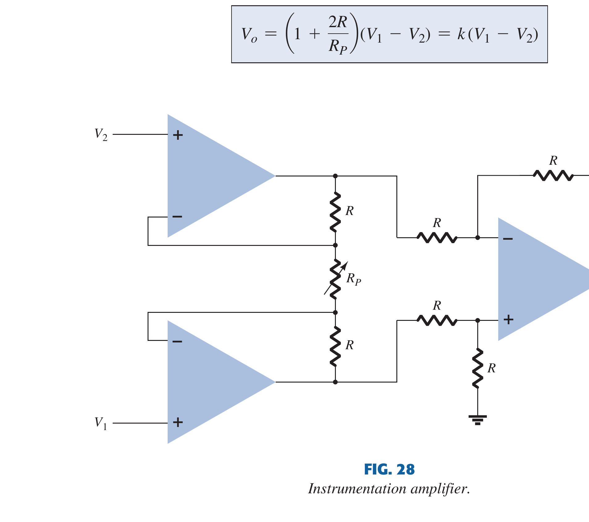
Book-grounded scoring points

The two input op-amps buffer both sources, so neither sensor is loaded appreciably.
One bridge resistor sets the first-stage differential gain; the final matched-resistor stage rejects common-mode voltage.
For the equal-$R$ textbook case, the first-stage factor is $1+2R/R_P$; resistor-ratio matching in the subtractor controls practical CMRR.

Source figure: Boylestad/Nashelsky, Electronic Devices and Circuit Theory (11th ed.), PDF p. 691.

Stage Operation¶

Input stage $A_1,A_2$
- both signals enter non-inverting inputs;
- input impedance is ideally very high;
- common-mode voltage is buffered;
- one resistor $R_{gain}$ controls differential gain.
Difference stage $A_3$
- subtracts the first-stage outputs;
- matched $R_3/R_2$ ratios determine gain and common-mode cancellation;
- converts the differential signal to a single-ended output.

For matched components,

\[ \boxed{ V_o=\left(1+\frac{2R_1}{R_{gain}}\right) \frac{R_3}{R_2}(V_2-V_1) }. \]

Why It Outperforms a Single Difference Amplifier¶

Very high input impedance at both inputs.
Gain adjusted by one resistor without disturbing final-stage ratio matching.
High CMRR when both signal paths and resistor ratios are matched.
Suitable for small differential signals riding on a large common-mode voltage.

Practical Limits¶

Resistor-ratio error in the difference stage reduces CMRR.
Input common-mode and output swing must stay inside supply limits.
Source imbalance converts input bias current into differential error.
Gain-bandwidth and slew rate decrease usable bandwidth at high gain.
Input noise and drift may dominate microvolt-level measurements.

Applications include strain gauges, RTDs, thermocouples, ECG/EEG electrodes, shunt-current sensing and data-acquisition front ends.

Op-Amp Configurations¶

Inverting Amplifier¶

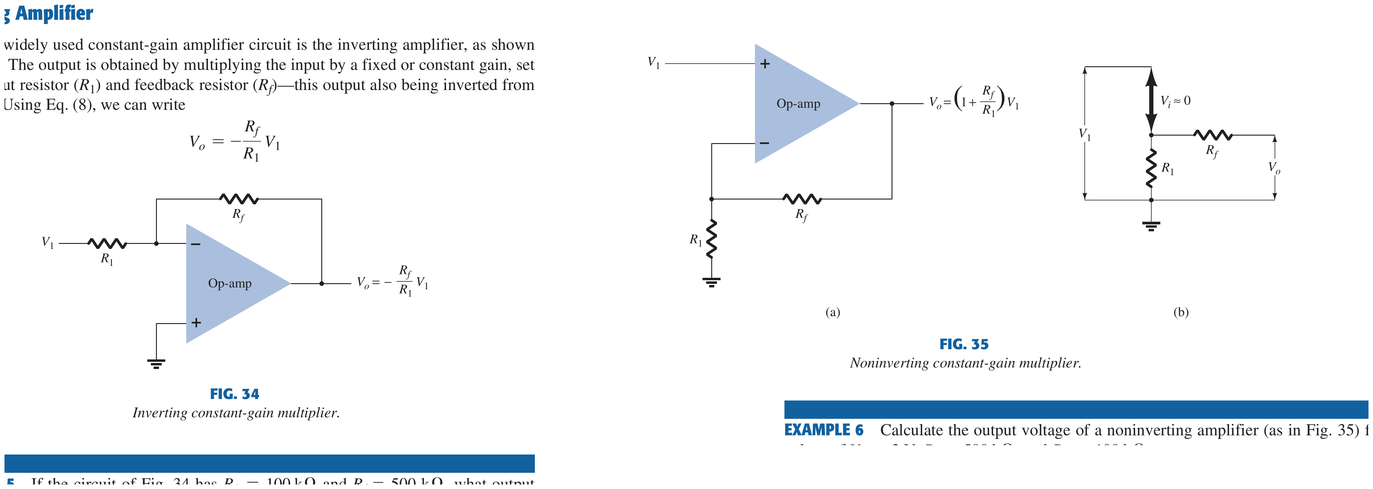
The input signal is applied to the inverting input ($V^-$) through resistor $R_1$. A feedback resistor $R_f$ connects the output back to the inverting input.

\[ \boxed{A_v = \frac{V_{out}}{V_{in}} = -\frac{R_f}{R_1}} \]

Negative sign indicates $180°$ phase inversion.
Input impedance: $Z_{in} = R_1$ (virtual ground at inverting input).
Gain depends only on external resistors (not on op-amp parameters).

Non-Inverting Amplifier¶

The input signal is applied to the non-inverting input ($V^+$). Feedback is from output to inverting input through $R_f$ and $R_1$.

\[ \boxed{A_v = \frac{V_{out}}{V_{in}} = 1 + \frac{R_f}{R_1}} \]

No phase inversion; gain is always $\geq 1$.
Input impedance: Very high (ideally $\infty$).
Special case — Voltage Follower (Buffer): When $R_f = 0$ and $R_1 = \infty$: $A_v = 1$. Used for impedance matching.

Fig: Textbook inverting and non-inverting op-amp circuits with closed-loop gain relations

Summing Amplifier (Adder)¶

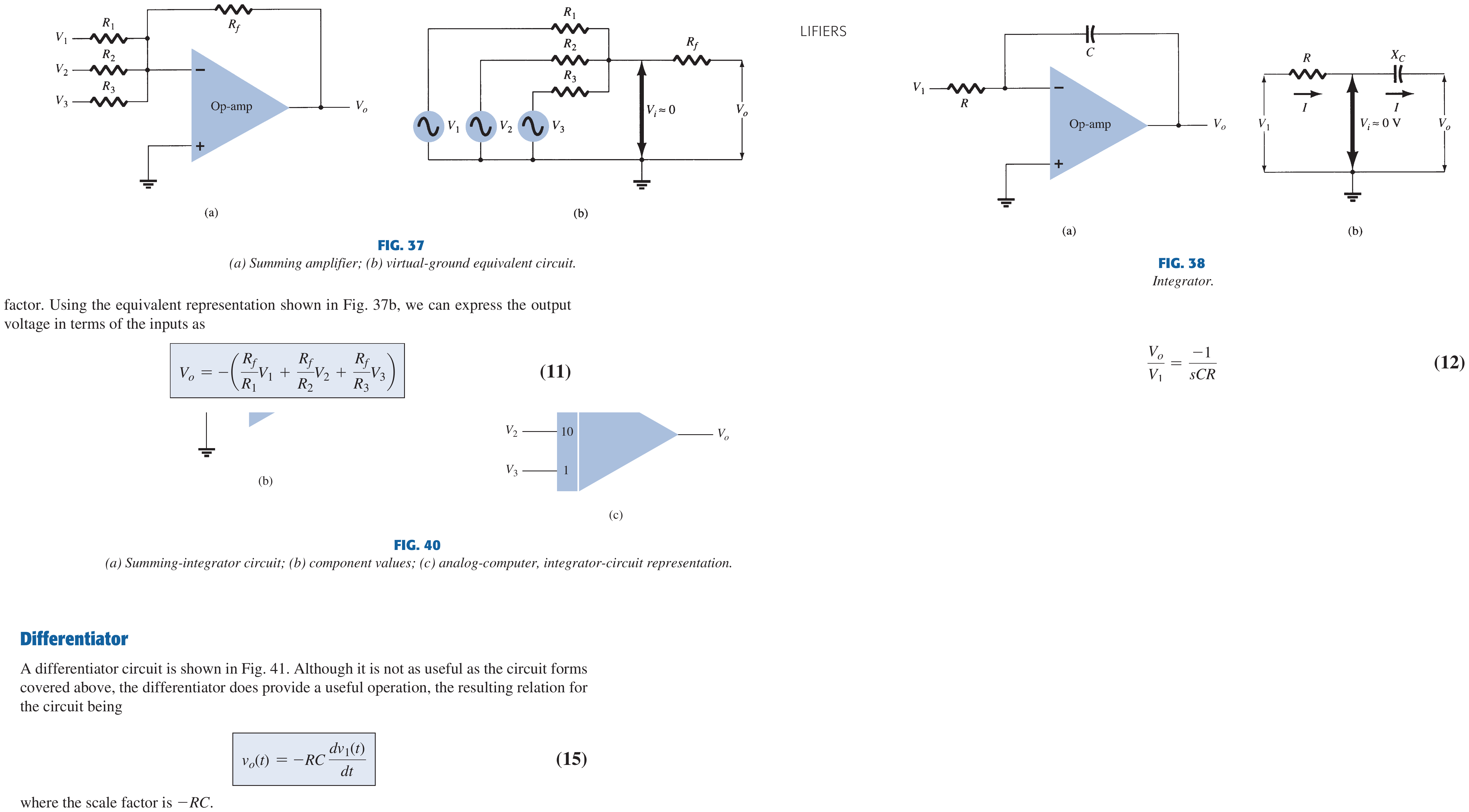
Multiple inputs are applied through separate input resistors to the inverting input:

\[ \boxed{V_{out} = -R_f\left(\frac{V_1}{R_1} + \frac{V_2}{R_2} + \frac{V_3}{R_3}\right)} \]

If all input resistors are equal ($R_1 = R_2 = R_3 = R$): $V_{out} = -\frac{R_f}{R}(V_1 + V_2 + V_3)$

Used in audio mixers, digital-to-analog converters, and weighted summing.

Difference (Differential) Amplifier¶

\[ \boxed{V_{out} = \frac{R_f}{R_1}(V_2 - V_1)} \quad \text{(when } R_1 = R_3 \text{ and } R_2 = R_f\text{)} \]

Amplifies only the difference between two inputs while rejecting common-mode signals.

Integrator¶

Replaces $R_f$ with a capacitor $C$:

\[ \boxed{V_{out}(t) = -\frac{1}{RC}\int_0^t V_{in}(\tau)\,d\tau} \]

Output is proportional to the time integral of the input. A square wave input produces a triangular wave output.

Differentiator¶

Replaces $R_1$ with a capacitor $C$:

\[ \boxed{V_{out}(t) = -RC\,\frac{dV_{in}(t)}{dt}} \]

Output is proportional to the rate of change of input. A triangular wave input produces a square wave output.

Fig: Textbook op-amp summing, integrating and differentiating circuits

Key Exam Points — Op-Amp

Ideal op-amp: infinite gain, infinite $Z_{in}$, zero $Z_{out}$, infinite bandwidth, infinite CMRR.
Virtual short: $V^+ = V^-$; Virtual ground: $V^- = 0$ (when $V^+$ is grounded).
Inverting gain = $-R_f/R_1$; Non-inverting gain = $1 + R_f/R_1$.
CMRR = $A_d/A_{cm}$ — measures ability to reject common-mode noise.
Slew rate limits maximum undistorted frequency: $f_{\max} = SR/(2\pi V_p)$.

Model Answer — Inverting and Non-Inverting Op-Amp Gains [5 marks]¶

Exam-ready answer

For an ideal op-amp operating linearly with negative feedback, $i^+=i^-=0$ and $V^+=V^-$. These two rules make the closed-loop gain depend on external resistors rather than the very large open-loop gain.

1. Inverting amplifier: $V^+$ is grounded, so $V^-=0$ by virtual ground. Applying KCL at the inverting node gives

\[ \frac{V_i-V^-}{R_1}=\frac{V^--V_o}{R_f}. \]

Putting $V^-=0$,

\[ \frac{V_i}{R_1}=-\frac{V_o}{R_f} \quad\Rightarrow\quad \boxed{A_v=\frac{V_o}{V_i}=-\frac{R_f}{R_1}}. \]

The minus sign means $180^\circ$ phase inversion, and the source sees $Z_{in}=R_1$.

2. Non-inverting amplifier: $V^+=V_i$, hence $V^-=V_i$. Since no current enters the input, $R_f$ and $R_1$ form an unloaded divider from $V_o$ to ground:

\[ V^-=V_o\frac{R_1}{R_1+R_f}=V_i. \]

Therefore

\[ \boxed{A_v=\frac{V_o}{V_i}=1+\frac{R_f}{R_1}}. \]

The output is in phase, gain cannot be below unity in this form, and input impedance is ideally infinite. With direct feedback ($R_f=0$ and $R_1$ omitted), $A_v=1$ and the circuit is a voltage follower used for impedance buffering.

Example: for $R_1=10\,\text{k}\Omega$ and $R_f=40\,\text{k}\Omega$, the inverting gain is $-4$, while the non-inverting gain is $+5$. A $0.2\,\text{V}$ input therefore gives $-0.8\,\text{V}$ or $+1.0\,\text{V}$ respectively, provided neither output exceeds the supply-limited swing and the signal lies within bandwidth/slew-rate limits.

Practice target: 8–9 minutes; draw both circuits and show the KCL/divider step before boxing each gain.

Model Answer — Op-Amp Summing, Differential, Integrator and Differentiator Circuits [10 marks]¶

Exam-ready answer

With an ideal op-amp under negative feedback, input currents are zero and $V^+=V^-$. Changing the input and feedback impedances around the inverting stage produces algebraic addition, subtraction, integration and differentiation.

1. Inverting summing amplifier: inputs $V_1,V_2,\ldots,V_n$ feed the virtual-ground node through $R_1,R_2,\ldots,R_n$, with feedback $R_f$. KCL gives

\[ \sum_{k=1}^{n}\frac{V_k}{R_k}=-\frac{V_o}{R_f} \quad\Rightarrow\quad \boxed{V_o=-R_f\sum_{k=1}^{n}\frac{V_k}{R_k}}. \]

Equal $R_k=R$ give a scaled sum $V_o=-(R_f/R)\sum V_k$; unequal resistors give a weighted sum. For example, $R_f=20\,\text{k}\Omega$, $R_1=10\,\text{k}\Omega$, $R_2=20\,\text{k}\Omega$, $V_1=0.5\,\text{V}$ and $V_2=1\,\text{V}$ yield $V_o=-(2V_1+V_2)=-2\,\text{V}$. Uses: audio mixing and DACs.

2. Differential amplifier: one input $V_1$ is applied to the inverting path and $V_2$ to the non-inverting path. When resistor ratios are accurately matched,

\[ \frac{R_2}{R_1}=\frac{R_4}{R_3}=k, \qquad \boxed{V_o=k(V_2-V_1)}. \]

Equal common-mode components cancel ideally. Resistor-ratio mismatch converts common-mode voltage into error, so precision matched networks are used in sensor interfaces and instrumentation.

3. Integrator: use input resistor $R$ and feedback capacitor $C$. In the $s$ domain, $Z_f=1/(sC)$, hence

\[ \boxed{\frac{V_o(s)}{V_i(s)}=-\frac{1}{sRC}}, \qquad \boxed{V_o(t)=V_o(0)-\frac{1}{RC}\int_0^t V_i(\tau)\,d\tau}. \]

A constant or square input produces a linear ramp or triangular output with slope $dV_o/dt=-V_i/(RC)$. An ideal integrator has infinite DC gain and drifts into saturation from offsets; a large resistor in parallel with $C$ limits low-frequency gain. Uses: waveform generation, analog computation and active filters.

4. Differentiator: use input capacitor $C$ and feedback resistor $R$. The capacitor current $i=C\,dV_i/dt$ flows through $R$, giving

\[ \boxed{\frac{V_o(s)}{V_i(s)}=-sRC}, \qquad \boxed{V_o(t)=-RC\frac{dV_i(t)}{dt}}. \]

A ramp/triangular input gives a constant/square output; a step ideally gives a narrow pulse. Since gain magnitude $|H(j\omega)|=\omega RC$ rises with frequency, an ideal differentiator strongly amplifies noise and may become unstable. A practical circuit adds a series input resistor and a small feedback capacitor to bound the useful frequency band. Uses: edge detection, pulse shaping and rate-of-change measurement.

Circuit	Mathematical action	Main practical limitation
Summer	Weighted addition	Output range and resistor accuracy
Differential	Subtraction/common-mode rejection	Ratio matching determines CMRR
Integrator	$1/s$ operation	Offset-driven DC saturation
Differentiator	$s$ operation	High-frequency noise and stability

All formulas assume linear operation; finite gain-bandwidth, slew rate, output-current capacity and supply rails limit amplitude and frequency in real circuits.

Practice target: 16–18 minutes; draw all four circuits, derive each boxed relation, and state one application plus one practical limitation.

Model Answer — Types of Op-Amps [10 marks]¶

Exam-ready answer

Op-amps are classified by the performance parameter or function optimized in their internal design.

Type	Key feature	Typical application
General-purpose	Balanced moderate specifications and low cost	Basic amplifiers and active filters
High-speed	High GBW/slew rate and low settling time	Video, fast ADC drive and pulse circuits
Precision	Very low offset, drift, bias current and noise; high CMRR/PSRR	Bridge sensors and DC measurement
Power	High output current/voltage with protection and thermal design	Actuators, speakers and power control
Comparator	Fast open-loop switching and logic output	Threshold and zero-crossing detection
Norton	Amplifies input-current difference, often from one supply	Current-mode filters and oscillators
Instrumentation	High input impedance, accurate differential gain and high CMRR	Low-level sensor/biomedical signals
Isolation	Galvanic input-output barrier	High-side measurement and safety isolation

A Norton op-amp responds approximately to $I^+-I^-$ and is useful in current-mode, single-supply circuits. An isolation op-amp transfers signal optically, capacitively or magnetically while keeping grounds ohmically separate; isolation rating, leakage, CMRR and bandwidth are important.

An instrumentation amplifier normally uses two high-input-impedance non-inverting stages followed by a matched difference amplifier. A comparator only resembles an op-amp: it is optimized to switch open loop, whereas a linear op-amp is optimized for negative-feedback operation.

The best type is selected from signal level, required accuracy, bandwidth, load current, supply voltage, common-mode range, environment and cost rather than from gain alone.

Practice target: 16–18 minutes; classify at least seven types and give one defining specification plus one use for each.

Model Answer — Three-Op-Amp Instrumentation Amplifier [5 marks]¶

Exam-ready answer

A three-op-amp instrumentation amplifier accurately amplifies a small differential signal in the presence of a large common-mode voltage.

$A_1$ and $A_2$ are non-inverting input stages, so both sources see very high input impedance. Their inverting nodes are joined by $R_{gain}$; changing this single resistor sets first-stage differential gain without loading the sources. $A_3$ is a matched-resistor difference amplifier that rejects the remaining common-mode component and gives a single-ended output.

For the resistor labels shown,

$$ \boxed{ V_o=\left(1+\frac{2R_1}{R_{gain}}\right) \frac{R_3}{R_2}(V_2-V_1) }. $$

Its advantages are high input impedance, gain control with one resistor and high CMRR. Final-stage resistor-ratio mismatch, input offset/bias current, noise, common-mode range, output swing and finite bandwidth limit practical accuracy. Applications include strain gauges, thermocouples, ECG/EEG, shunt-current measurement and data acquisition.

Practice target: 9 minutes; draw all three op-amps, identify the two stages, box the gain and state that resistor-ratio matching determines practical CMRR.

Mind Map¶

Mind map

Open the interactive mind map for operational amplifiers →