System Equations and Digital Filters¶

Possible Exam Questions¶

Exam Questions and Answer Map

Evidence note: [PYQ paper/year] = exact question observed in that past paper; [likely] = pattern-predicted variant not confirmed as exact PYQ.

Explain the solution of systems described by differential/difference equations. [5] — [likely]
Answer plan: Write general N-th order LCCDE → take Laplace/z-transform → obtain transfer function \(H(s)\) or \(H(z)\) → solve for output via partial fractions and inverse transform → distinguish zero-input and zero-state response.
Model answer: Solving Differential and Difference Equations
Differentiate FIR and IIR filters (stability, phase, implementation). [5] — [likely]
Answer plan: Define FIR (finite impulse response, no feedback) vs IIR (infinite, uses feedback) → compare: FIR always stable and can be linear-phase; IIR may be unstable but is more efficient (fewer coefficients for same selectivity) → list realization forms → mention applications.
Model answer: FIR and IIR Filter Comparison
Explain the realization of digital filters (direct form I and II). [5] — [likely]
Answer plan: Draw Direct Form I (separate FIR and IIR sections, needs 2N delays) → draw Direct Form II (canonic, shares delay elements, needs N delays) → label coefficients \(a_k\), \(b_k\) → state advantage of DF-II (fewer memory elements).
Model answer: Direct Form I and II Realizations

1. Differential Equations¶

Likely Exam Question (5 marks)

"Represent a continuous-time LTI system by a differential equation and explain its solution."

Continuous-Time Differential Equation¶

A continuous-time LTI system can be represented by:

\[ \boxed{\sum_{k=0}^{N}a_k\frac{d^k y(t)}{dt^k} = \sum_{m=0}^{M}b_m\frac{d^m x(t)}{dt^m}} \]

where \(a_k\) and \(b_m\) are constant coefficients.

Transfer Function¶

Taking Laplace transform with zero initial conditions:

\[ \boxed{H(s) = \frac{Y(s)}{X(s)} = \frac{\sum_{m=0}^{M}b_ms^m}{\sum_{k=0}^{N}a_ks^k}} \]

The poles and zeros of \(H(s)\) determine system behavior, stability, and frequency response.

With non-zero initial conditions, the total response has two parts:

\[ \boxed{y(t)=y_{zi}(t)+y_{zs}(t)} \]

The zero-input response \(y_{zi}(t)\) is caused by stored initial energy with the external input set to zero.
The zero-state response \(y_{zs}(t)\) is caused by the applied input with all initial conditions set to zero. It equals \(x(t)*h(t)\).

The transfer function describes only the zero-state response because it is defined using zero initial conditions.

Frequency Response¶

For sinusoidal steady-state analysis:

\[ \boxed{H(j\omega) = H(s)\big|_{s=j\omega}} \]

If input is \(x(t)=A\cos(\omega t)\), output is a sinusoid at the same frequency with changed amplitude and phase.

Solved First-Order Continuous-Time System¶

Consider

\[ \frac{dy(t)}{dt}+ay(t)=bx(t), \qquad a>0 \]

With zero initial condition, taking the Laplace transform gives

\[ (s+a)Y(s)=bX(s) \]

Therefore,

\[ \boxed{H(s)=\frac{Y(s)}{X(s)}=\frac{b}{s+a}} \]

The system has one pole at \(s=-a\), and its impulse response is

\[ \boxed{h(t)=be^{-at}u(t)} \]

Because \(a>0\), the pole is in the open left half-plane and \(h(t)\) is absolutely integrable, so the causal system is BIBO stable.

For a unit-step input \(x(t)=u(t)\) and initial value \(y(0^-)=y_0\), the unilateral Laplace transform gives

\[ (s+a)Y(s)=\frac{b}{s}+y_0 \]

Hence

\[ Y(s)=\underbrace{\frac{y_0}{s+a}}_{\text{zero-input}} +\underbrace{\frac{b}{s(s+a)}}_{\text{zero-state}} \]

and

\[ \boxed{y(t)=\left[y_0e^{-at}+\frac{b}{a}\left(1-e^{-at}\right)\right]u(t)} \]

The transient terms decay with time constant \(1/a\), and the final value is \(b/a\).

2. Difference Equations¶

Likely Exam Question (5 marks)

"Write the difference equation of a digital filter and obtain its system function."

Discrete-Time Difference Equation¶

A discrete-time LTI system can be described by a linear constant-coefficient difference equation:

\[ \boxed{y[n] + \sum_{k=1}^{N}a_ky[n-k] = \sum_{m=0}^{M}b_mx[n-m]} \]

This equation directly maps to a digital filter structure.

System Function¶

Taking Z transform with zero initial conditions:

\[ \boxed{H(z) = \frac{Y(z)}{X(z)} = \frac{\sum_{m=0}^{M}b_mz^{-m}}{1 + \sum_{k=1}^{N}a_kz^{-k}}} \]

Frequency response is obtained by evaluating on the unit circle:

\[ \boxed{H(e^{j\Omega}) = H(z)\big|_{z=e^{j\Omega}}} \]

This frequency response exists only when the Z-transform ROC includes the unit circle.

As in continuous time, the total response is the sum of the zero-input response caused by initial stored values and the zero-state response caused by the external input. The system function \(H(z)\) describes the zero-state response.

Solved First-Order Discrete-Time System¶

Consider the causal difference equation

\[ y[n]-ay[n-1]=bx[n], \qquad \lvert a\rvert<1 \]

With zero initial condition,

\[ Y(z)-az^{-1}Y(z)=bX(z) \]

so

\[ \boxed{H(z)=\frac{b}{1-az^{-1}}} \]

and

\[ \boxed{h[n]=ba^nu[n]} \]

The pole is at \(z=a\). Since \(\lvert a\rvert<1\), the pole lies strictly inside the unit circle and the causal system is BIBO stable.

For \(x[n]=u[n]\) with zero initial condition,

\[ y_{zs}[n]=b\sum_{k=0}^{n}a^k =\boxed{\frac{b(1-a^{n+1})}{1-a}u[n]} \]

If \(y[-1]=y_{-1}\) is non-zero, the zero-input response is

\[ y_{zi}[n]=a^{n+1}y_{-1}u[n] \]

and the total response is \(y[n]=y_{zi}[n]+y_{zs}[n]\).

3. Digital Filters¶

Likely Exam Question (10 marks)

"Compare FIR and IIR filters. State their advantages, disadvantages, and applications."

Digital Filter Definition¶

A digital filter processes discrete-time signals to modify their frequency content. It may pass desired frequencies and attenuate undesired frequencies.

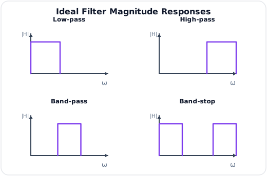
Common filter types:

Low-pass filter: passes low frequencies
High-pass filter: passes high frequencies
Band-pass filter: passes a band of frequencies
Band-stop filter: rejects a band of frequencies

Fig: Ideal magnitude responses of low-pass, high-pass, band-pass and band-stop filters

4. FIR Filters¶

FIR Definition¶

An FIR (Finite Impulse Response) filter has an impulse response of finite duration. Its output depends only on present and past input samples.

\[ \boxed{y[n] = \sum_{k=0}^{M}b_kx[n-k]} \]

System function:

\[ \boxed{H(z)=\sum_{k=0}^{M}b_kz^{-k}} \]

Fig: FIR direct-form (transversal) structure: a tapped delay line of z⁻¹ blocks, coefficient multipliers bₖ, and a summing chain giving y[n]

This tapped-delay-line (transversal) structure has no feedback path, so an FIR filter is always stable.

FIR Characteristics¶

Non-recursive structure
Always BIBO stable if coefficients are finite
Can have exactly linear phase
Usually requires higher order than IIR for sharp cutoff
No feedback, so round-off error accumulation is low

FIR Applications¶

Linear-phase audio processing
Data communication pulse shaping
Moving-average smoothing
Systems where stability must be guaranteed

5. IIR Filters¶

IIR Definition¶

An IIR (Infinite Impulse Response) filter has an impulse response that theoretically continues forever. Its output depends on present input, past inputs, and past outputs.

\[ \boxed{y[n] = \sum_{m=0}^{M}b_mx[n-m] - \sum_{k=1}^{N}a_ky[n-k]} \]

System function:

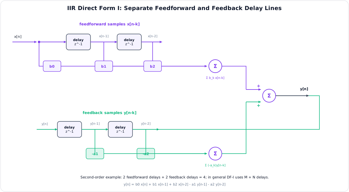
\[ \boxed{H(z) = \frac{\sum_{m=0}^{M}b_mz^{-m}}{1 + \sum_{k=1}^{N}a_kz^{-k}}} \]

Direct Form Realization (I and II)¶

The system function can be drawn as a network of delays (\(z^{-1}\)), multipliers and adders. Two standard realizations are:

Direct Form I — the feedforward (numerator \(b_m\)) and feedback (denominator \(a_k\)) parts are implemented as two separate sections in cascade, each with its own delay line (\(M+N\) delays total).
Direct Form II (canonical) — reordering the two sections lets both delay lines hold the same intermediate signal \(w[n]\), so they merge into one delay line using only \(\max(M,N)\) delays — the minimum possible, hence "canonical".

For Direct Form I, the realizable equation is the original difference equation:

\[ \boxed{y[n]=\sum_{m=0}^{M}b_mx[n-m] -\sum_{k=1}^{N}a_ky[n-k]} \]

The samples \(x[n-m]\) occupy the feedforward delay line and \(y[n-k]\) occupy a separate feedback delay line.

For Direct Form II, define the internal state \(w[n]\):

\[ \boxed{w[n]=x[n]-\sum_{k=1}^{N}a_kw[n-k]} \]

\[ \boxed{y[n]=\sum_{m=0}^{M}b_mw[n-m]} \]

Both sums use the same stored delayed values of \(w[n]\), which is why only one delay line is needed. Missing coefficients are treated as zero when \(M\neq N\).

Fig: IIR Direct Form I with separate feedforward and feedback delay lines, coefficient taps and output summer

Fig: IIR Direct Form II: a shared central delay line holding w[n], feedback coefficients −aₖ on the left, feedforward coefficients bₖ on the right, combined at input and output summers

Both forms realize the identical \(H(z)\); DF-II minimises memory, while DF-I can avoid overflow at the shared internal node.

IIR Characteristics¶

Recursive structure with feedback
Efficient for sharp cutoff using lower order
For a causal rational IIR filter, BIBO stability requires every pole to lie strictly inside the unit circle; a pole on or outside it causes instability
Exact linear phase is generally not possible
Often designed from analog prototype filters such as Butterworth or Chebyshev
More sensitive than FIR filters to coefficient quantization, round-off error, and limit-cycle oscillations

IIR Applications¶

Low-order real-time audio equalizers and tone controls
Speech and communication-channel filtering where computation is limited
Biomedical low-pass, high-pass, and notch filters
Recursive smoothing and sensor-data conditioning
Digital implementations derived from Butterworth, Chebyshev, and elliptic analog prototypes

The main advantage of an IIR filter is that a sharp transition can be obtained with fewer coefficients, delays, and multiplications. Its main disadvantages are possible instability, nonlinear phase, and greater sensitivity to finite-word-length effects.

FIR vs IIR Comparison¶

Feature	FIR Filter	IIR Filter
Impulse response	Finite duration	Infinite duration
Structure	Non-recursive	Recursive
Feedback	No feedback	Uses feedback
Stability	Always stable for finite coefficients	Depends on pole locations
Phase	Exact linear phase possible	Usually nonlinear phase
Order for sharp cutoff	Higher	Lower
Computation	More multiplications	Fewer multiplications

Solved Example - Moving Average FIR¶

Q. Write the output equation of a 3-point moving average filter.

For equal coefficients:

\[ b_0=b_1=b_2=\frac{1}{3} \]

\[ \boxed{y[n] = \frac{1}{3}\left(x[n]+x[n-1]+x[n-2]\right)} \]

This is an FIR low-pass smoothing filter.

Key Exam Points - System Equations and Digital Filters

Differential equations model continuous-time LTI systems; take the Laplace transform to get \(H(s)\).
Difference equations model discrete-time LTI systems and digital filters; take the Z transform to get \(H(z)\).
Total response = zero-input (from initial conditions) + zero-state (\(x*h\)); \(H\) describes the zero-state part.
FIR: finite \(h\), no feedback, always stable, can be exactly linear phase.
IIR: infinite \(h\), uses feedback, efficient (low order) but stability depends on pole locations.
Direct Form II is canonical — it shares one delay line and uses the minimum number of delays.

Model Answer — Solving Differential and Difference Equations [5 marks]¶

Exam-ready answer

A CT LTI system is described by a linear constant-coefficient differential equation

\[ \sum_{k=0}^{N}a_k\frac{d^ky(t)}{dt^k} =\sum_{m=0}^{M}b_m\frac{d^mx(t)}{dt^m}. \]

With zero initial conditions, the Laplace transform converts differentiation into multiplication by \(s\):

\[ \boxed{H(s)=\frac{Y(s)}{X(s)} =\frac{\sum_{m=0}^{M}b_ms^m}{\sum_{k=0}^{N}a_ks^k}}. \]

A DT LTI system obeys

\[ y[n]+\sum_{k=1}^{N}a_ky[n-k] =\sum_{m=0}^{M}b_mx[n-m], \]

and, under zero initial conditions,

\[ \boxed{H(z)=\frac{Y(z)}{X(z)} =\frac{\sum_{m=0}^{M}b_mz^{-m}} {1+\sum_{k=1}^{N}a_kz^{-k}}}. \]

The solution procedure is: (1) transform the equation while inserting given initial conditions in unilateral LT/ZT formulas; (2) collect \(Y\); (3) write \(Y=HX\) for the zero-state part; (4) use partial fractions; and (5) inverse-transform with the proper ROC. The total response is

\[ \boxed{y=y_{zi}+y_{zs}}, \]

where \(y_{zi}\) is due to stored initial energy with \(x=0\), and \(y_{zs}=x*h\) is due to the input with zero initial conditions. A transfer function describes only \(y_{zs}\).

Worked CT example: for \(y'(t)+2y(t)=x(t)\), \(y(0^-)=0\), and \(x(t)=u(t)\),

\[ H(s)=\frac1{s+2},\qquad Y(s)=\frac1{s(s+2)}=\frac12\left(\frac1s-\frac1{s+2}\right), \]

so

\[ \boxed{y(t)=\tfrac12(1-e^{-2t})u(t)}. \]

The pole \(s=-2\) gives a decaying transient. For a causal rational DT system, poles strictly inside \(|z|=1\) ensure stability; in CT they must lie strictly in the open left half-plane. The frequency responses are obtained as \(H(j\omega)\) and \(H(e^{j\Omega})\) only when the corresponding ROC contains the evaluation contour.

Practice target: 10 minutes; show the transform, partial fractions, inverse result and clearly separate zero-input from zero-state response.

Model Answer — FIR and IIR Filter Comparison [5 marks]¶

Exam-ready answer

A digital filter maps input samples to output samples. An FIR filter has finitely many nonzero impulse-response samples and no output feedback:

\[ \boxed{y[n]=\sum_{k=0}^{M}b_kx[n-k]}, \qquad H(z)=\sum_{k=0}^{M}b_kz^{-k}. \]

Fig: FIR tapped-delay-line realization with feedforward coefficient taps

An IIR filter is recursive; past outputs feed back and generally produce an impulse response of infinite duration:

\[ \boxed{y[n]=\sum_{m=0}^{M}b_mx[n-m]-\sum_{k=1}^{N}a_ky[n-k]}, \]

\[ H(z)=\frac{\sum_{m=0}^{M}b_mz^{-m}} {1+\sum_{k=1}^{N}a_kz^{-k}}. \]

Fig: Canonical IIR Direct Form II realization with feedforward and feedback coefficients

Feature	FIR	IIR
Feedback	absent, nonrecursive	present, recursive
Stability	always BIBO stable for finite coefficients	stable only when the ROC includes the unit circle; causal rational case requires all poles inside it
Phase	exact linear phase possible with symmetric/antisymmetric coefficients	generally nonlinear phase
Order for a sharp transition	usually higher	usually lower and computationally efficient
Finite-word effects	low sensitivity, no limit cycles from feedback	more coefficient-sensitive; round-off and limit cycles possible
Typical use	pulse shaping, audio with phase fidelity, moving average	low-order equalizers, notch filters, sensor smoothing

For example, the three-point moving-average FIR has \(b_0=b_1=b_2=1/3\) and

\[ y[n]=\frac{x[n]+x[n-1]+x[n-2]}3. \]

Its finite impulse response is \(\{1/3,1/3,1/3\}\) and is absolutely summable. By contrast, \(H(z)=1/(1-az^{-1})\) has \(h[n]=a^nu[n]\); it is a causal stable IIR only when \(|a|<1\). Hence FIR is preferred for guaranteed stability and linear phase, whereas IIR is preferred when low order and sharp selectivity dominate.

Practice target: 9 minutes; write both equations, compare at least six features, and state the pole condition rather than merely saying that IIR “may be unstable.”

Model Answer — Direct Form I and II Realizations [5 marks]¶

Exam-ready answer

For the normalized IIR transfer function

\[ H(z)=\frac{b_0+b_1z^{-1}+\cdots+b_Mz^{-M}} {1+a_1z^{-1}+\cdots+a_Nz^{-N}}, \]

the realizable difference equation is

\[ \boxed{y[n]=\sum_{m=0}^{M}b_mx[n-m] -\sum_{k=1}^{N}a_ky[n-k]}. \]

Direct Form I (DF-I) implements the numerator and denominator as separate feedforward and feedback sections. One delay line stores \(x[n-m]\) and another stores \(y[n-k]\), so it uses \(M+N\) delay elements, \(M+N+1\) multipliers, and the required adders. Its separate internal paths often provide better control of overflow.

Fig: IIR Direct Form I with separate input and output delay lines

Direct Form II (DF-II) interchanges the cascade order and shares one state sequence. Define

\[ \boxed{w[n]=x[n]-\sum_{k=1}^{N}a_kw[n-k]}, \]

\[ \boxed{y[n]=\sum_{m=0}^{M}b_mw[n-m]}. \]

Both sums use the same delayed \(w\) samples, so only \(\max(M,N)\) delays are needed; absent higher-order coefficients are zero. This is the canonical realization because it uses the minimum memory.

Fig: IIR Direct Form II with a shared state delay line

Point	Direct Form I	Direct Form II
Delay lines	two separate	one shared
Delay count	\(M+N\)	\(\max(M,N)\)
Transfer function	identical \(H(z)\)	identical \(H(z)\)
Numerical issue	larger memory, often less internal-node overflow	memory efficient, but internal \(w[n]\) can have large dynamic range

As a second-order example, \(H(z)=(b_0+b_1z^{-1}+b_2z^{-2})/(1+a_1z^{-1}+a_2z^{-2})\) needs four delays in DF-I but only two in DF-II. Neither structure changes poles or stability; for a causal rational filter, BIBO stability still requires every pole strictly inside the unit circle.

Practice target: 10 minutes; draw both labeled structures, write the \(w[n]\) equations and state the exact delay counts and numerical trade-off.

Mind Map¶

Mind map

Open the interactive mind map for this chapter →