Fourier, Laplace and Z Transforms¶
Possible Exam Questions¶
Exam Questions and Answer Map
Evidence note: [PYQ paper/year] = exact question observed in that past paper; [likely] = pattern-predicted variant not confirmed as exact PYQ.
-
Distinguish between Fourier transform, Laplace transform and z-transform. [4] — [PYQ 2079]
-
Answer plan: State each transform's definition and domain (FT: time→frequency for stable signals; LT: adds convergence factor \(e^{-\sigma t}\) for transient analysis; ZT: discrete-time equivalent of LT) → compare ROC requirements → tabulate applicability (signal type, analysis purpose).
-
Model answer: Fourier, Laplace and z-Transform Comparison
-
Find the Fourier transform of the impulse (delta) function. [4] — [PYQ 2079]
-
Answer plan: Write FT integral \(\int_{-\infty}^{\infty}\delta(t)e^{-j\omega t}dt\) → apply sifting property → obtain \(X(\omega)=1\) → interpret: impulse contains all frequencies equally (flat spectrum).
-
Model answer: Fourier Transform of the Unit Impulse
-
State and prove the important properties of the Fourier transform. [5–10] — [likely]
-
Answer plan: List linearity, time-shift, frequency-shift, scaling, differentiation, convolution, Parseval's → prove at least time-shift and convolution property using the integral definition → state duality.
-
Model answer: Fourier-Transform Properties and Proofs
-
Explain the Hilbert transform and its application in SSB generation. [5] — [likely]
-
Answer plan: Define Hilbert transform as \(-90°\) phase shift of all frequency components → write \(\hat{x}(t)=x(t)*\frac{1}{\pi t}\) → define analytic signal \(x_a(t)=x(t)+j\hat{x}(t)\) → show one-sided spectrum → apply to SSB: multiply message by \(\cos\omega_c t\) and Hilbert of message by \(\sin\omega_c t\).
-
Model answer: Hilbert Transform and SSB Generation
-
State the properties of the z-transform; find the z-transform of a standard sequence. [5] — [likely]
-
Answer plan: Define \(X(z)=\sum x[n]z^{-n}\) → list linearity, time-shift, convolution, initial/final value theorems → state ROC significance → compute ZT of \(a^n u[n] \to \frac{1}{1-az^{-1}}\), ROC \(|z|>|a|\).
-
Model answer: z-Transform Properties and Standard Sequence
-
Distinguish the four Fourier representations (FS, FT, DTFT, DFT). [5] — [likely]
-
Answer plan: Classify by continuous/discrete time × periodic/aperiodic → FS (CT periodic, discrete spectrum), FT (CT aperiodic, continuous spectrum), DTFT (DT aperiodic, continuous \(2\pi\)-periodic spectrum), DFT (DT finite, discrete spectrum) → note Laplace/Z generalise FT/DTFT.
-
Model answer: Fourier Series, FT, DTFT and DFT
-
State the sampling theorem; explain aliasing and reconstruction. [5] — [likely]
-
Answer plan: State \(f_s\ge 2f_m\) → explain spectrum replication every \(f_s\) → aliasing when \(f_s<2f_m\) (use anti-alias LPF) → reconstruct with an ideal LPF / sinc interpolation.
- Model answer: Sampling Theorem, Aliasing and Reconstruction
1. Fourier Series¶
Likely Exam Question (5 marks)
"State Fourier series representation of a periodic signal and define its coefficients."
Fourier Series Definition¶
Any periodic signal \(x(t)\) with period \(T_0\) and fundamental angular frequency \(\omega_0 = 2\pi/T_0\) can be represented as a sum of harmonically related sinusoids.
Complex Exponential Fourier Series¶
where Fourier coefficients are:
The integral may be evaluated over any one complete period; its value is independent of the chosen starting point \(t_0\).
Trigonometric Fourier Series¶
For this convention, the coefficients are
Here \(a_0\) is the average (DC) value, while \(a_n\) and \(b_n\) give the cosine and sine content of the \(n\)th harmonic. These formulas follow from the orthogonality of distinct sine and cosine harmonics over one complete period: multiplying the series by the required basis function and integrating eliminates all other harmonics.
Symmetry Rules¶
| Signal Symmetry | Fourier Series Result |
|---|---|
| Even signal | Only cosine terms, \(b_n = 0\) |
| Odd signal | Only sine terms, \(a_0 = a_n = 0\) |
| Half-wave symmetry | No even harmonics |
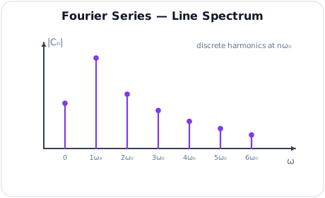
A periodic signal has a discrete (line) spectrum — energy appears only at \(0, \omega_0, 2\omega_0, \dots\)
Convergence (Dirichlet Conditions) and the Gibbs Phenomenon¶
A Fourier series converges to \(x(t)\) when the Dirichlet conditions hold over one period: \(x(t)\) is absolutely integrable, has a finite number of maxima and minima, and a finite number of finite discontinuities. At a jump discontinuity the series converges to the midpoint of the jump. Near such a jump the truncated series always overshoots by about 9% of the jump height no matter how many harmonics are summed — this persistent ripple is the Gibbs phenomenon.
2. Fourier Transform¶
Likely Exam Question (10 marks)
"Define Fourier transform. State important properties and common transform pairs."
Fourier Transform Definition¶
The Fourier transform represents an aperiodic signal in terms of its continuous frequency components.
Forward transform:
Inverse transform:
Physical Meaning¶
- \(x(t)\) describes how a signal varies with time.
- \(X(\omega)\) describes how much of each frequency is present.
- Magnitude spectrum: \(\lvert X(\omega)\rvert\)
- Phase spectrum: \(\angle X(\omega)\)
Important Properties¶
| Property | Time Domain | Frequency Domain |
|---|---|---|
| Linearity | \(ax_1(t)+bx_2(t)\) | \(aX_1(\omega)+bX_2(\omega)\) |
| Time shift | \(x(t-t_0)\) | \(e^{-j\omega t_0}X(\omega)\) |
| Frequency shift | \(e^{j\omega_0t}x(t)\) | \(X(\omega-\omega_0)\) |
| Time scaling | \(x(at)\) | \(\frac{1}{\lvert a\rvert}X(\omega/a)\) |
| Differentiation | \(\frac{d x(t)}{dt}\) | \(j\omega X(\omega)\) |
| Convolution | \(x(t)*h(t)\) | \(X(\omega)H(\omega)\) |
| Multiplication | \(x(t)g(t)\) | \(\frac{1}{2\pi}X(\omega)*G(\omega)\) |
| Duality | \(X(t)\) | \(2\pi x(-\omega)\) |
| Conjugate symmetry (\(x\) real) | \(x(t)\) | \(X(-\omega)=X^*(\omega)\) |
| Parseval (energy) | \(\int\lvert x(t)\rvert^2dt\) | \(\frac{1}{2\pi}\int\lvert X(\omega)\rvert^2d\omega\) |
Compact Proofs of Important Properties¶
Assume \(x(t)\leftrightarrow X(\omega)\) and that the required integrals and boundary terms exist.
1. Linearity¶
Because integration is linear,
2. Time Shifting¶
Let \(\tau=t-t_0\). Then
A time delay therefore changes phase but not magnitude.
3. Frequency Shifting¶
Multiplication by a complex carrier translates the spectrum by \(\omega_0\); this is the mathematical basis of modulation.
4. Time Scaling¶
With \(\tau=at\) and accounting for reversal of the integration limits when \(a<0\),
Thus compression in time produces expansion in frequency, and vice versa.
5. Differentiation in Time¶
Integration by parts gives
where the boundary term is zero for a suitably decaying signal.
6. Convolution¶
For \(y(t)=x(t)*h(t)\),
where \(\lambda=t-\tau\). Consequently, a difficult time-domain convolution becomes simple multiplication in the frequency domain.
7. Duality¶
Because the forward and inverse transforms differ only by a sign and a \(2\pi\) factor, every pair has a dual:
For example, \(\delta(t)\leftrightarrow 1\) has the dual \(1\leftrightarrow 2\pi\delta(\omega)\), and a rectangular pulse ↔ sinc has the dual sinc ↔ rectangle. Duality halves the number of pairs you must memorise.
8. Parseval's (Rayleigh) Energy Theorem¶
Total energy is the same whether computed in time or frequency:
Here \(\lvert X(\omega)\rvert^2\) is the energy spectral density (ESD) — energy per unit angular frequency. The theorem lets energy be evaluated in whichever domain is easier.
9. Conjugate Symmetry of Real Signals¶
If \(x(t)\) is real, its spectrum is Hermitian:
so the magnitude \(\lvert X(\omega)\rvert\) is even and the phase \(\angle X(\omega)\) is odd. Consequently a real even signal has a purely real spectrum and a real odd signal a purely imaginary one — exactly why \(\cos\omega_0 t\) produces real impulses while \(\sin\omega_0 t\) produces imaginary ones.
Short Application¶
Since
the time-shift property immediately gives
The delay \(t_0\) adds linear phase \(-\omega t_0\) but leaves the magnitude spectrum unchanged.
Common Transform Pairs¶
| Time Signal | Fourier Transform |
|---|---|
| \(\delta(t)\) | \(1\) |
| \(1\) | \(2\pi\delta(\omega)\) |
| \(e^{-at}u(t)\), \(a>0\) | \(\frac{1}{a+j\omega}\) |
| \(\cos\omega_0t\) | \(\pi[\delta(\omega-\omega_0)+\delta(\omega+\omega_0)]\) |
| \(\sin\omega_0t\) | \(\frac{\pi}{j}[\delta(\omega-\omega_0)-\delta(\omega+\omega_0)]\) |
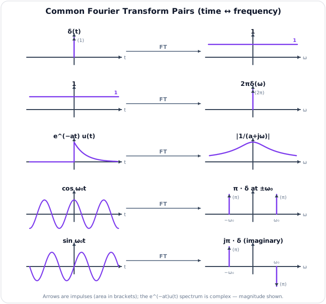
Each row shows a signal and its spectrum: an impulse ↔ a flat spectrum, a constant ↔ an impulse at \(\omega=0\), a decaying exponential ↔ a smooth low-pass magnitude, and cosine/sine ↔ line spectra at \(\pm\omega_0\) (real for cosine, imaginary for sine).
3. Hilbert Transform¶
Likely Exam Question (5 marks)
"What is Hilbert transform? State its frequency-domain property and explain its use in SSB generation."
Hilbert Transform Definition¶
The Hilbert transform of \(x(t)\) is:
where \(\operatorname{p.v.}\) denotes Cauchy principal value.
Frequency-Domain Interpretation¶
If \(x(t) \leftrightarrow X(\omega)\), then:
Thus Hilbert transform shifts:
- Positive frequency components by \(-90^\circ\)
- Negative frequency components by \(+90^\circ\)
Analytic Signal¶
For a real signal \(x(t)\), the analytic signal has no negative-frequency components. It is useful for envelope detection, instantaneous amplitude and phase, and single-sideband modulation.
Application in SSB Generation¶
In the phase-shift method of SSB generation, the message \(m(t)\) is divided into two paths. One path is used directly, while the other passes through a Hilbert transformer to produce \(\hat m(t)\), which is in phase quadrature with \(m(t)\). The two paths modulate quadrature carriers and are then added or subtracted:
To see the sideband cancellation, let \(m(t)=\cos\omega_mt\). Since the adopted Hilbert-transform convention gives \(\hat m(t)=\sin\omega_mt\),
whereas
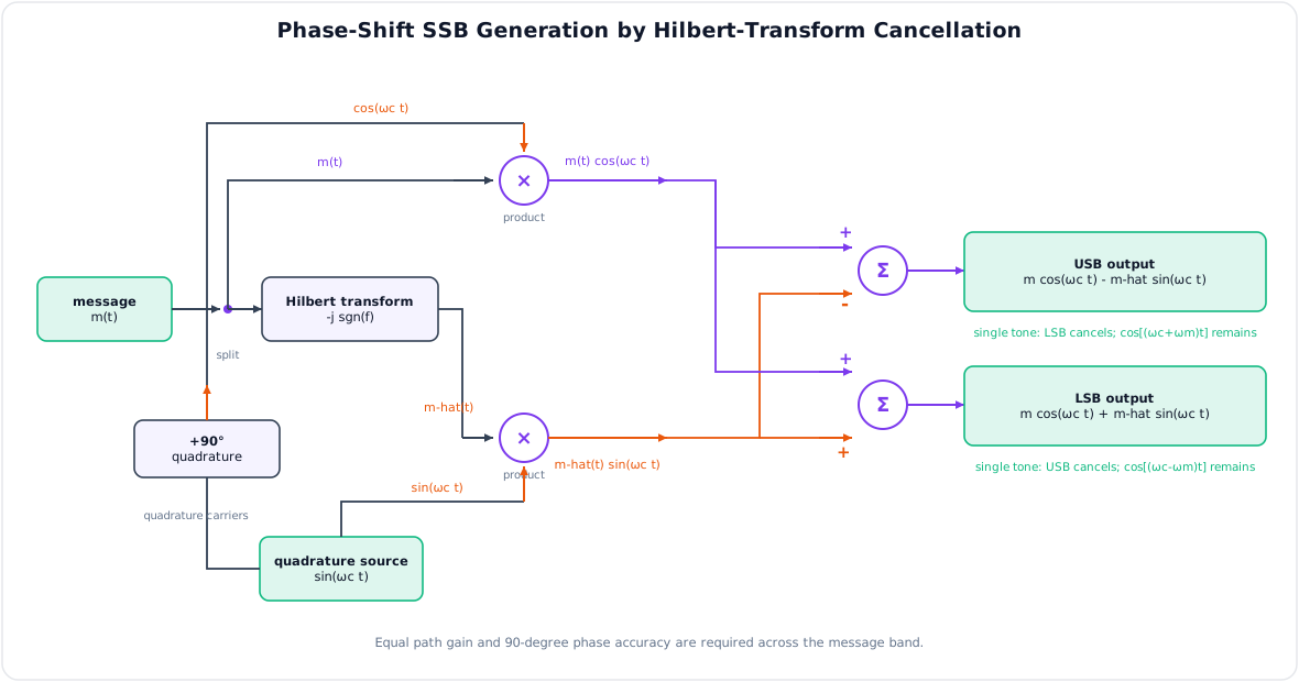
Thus one sideband reinforces while the other cancels. SSB transmits the information using only half the bandwidth of conventional AM and avoids carrier-power transmission.
4. Z Transform¶
Likely Exam Question (10 marks)
"Define Z transform. Explain ROC, causality, stability, and relation with DTFT."
Z-Transform Definition¶
The Z transform of a discrete-time signal \(x[n]\) is:
where \(z\) is a complex variable.
Region of Convergence (ROC)¶
The ROC is the set of values of \(z\) for which the Z-transform sum converges. ROC is important because the same algebraic expression may represent different time sequences depending on ROC.
Common Z-Transform Pairs¶
| Sequence | Z Transform | ROC |
|---|---|---|
| \(\delta[n]\) | \(1\) | entire z-plane |
| \(u[n]\) | \(\frac{1}{1-z^{-1}}\) | \(\lvert z\rvert > 1\) |
| \(a^n u[n]\) | \(\frac{1}{1-az^{-1}}\) | \(\lvert z\rvert > \lvert a\rvert\) |
| \(-a^n u[-n-1]\) | \(\frac{1}{1-az^{-1}}\) | \(\lvert z\rvert < \lvert a\rvert\) |
Important Properties¶
If \(x[n]\leftrightarrow X(z)\) and \(y[n]\leftrightarrow Y(z)\), then:
| Property | Time-domain operation | Z-domain result |
|---|---|---|
| Linearity | \(ax[n]+by[n]\) | \(aX(z)+bY(z)\) |
| Time shift | \(x[n-n_0]\) | \(z^{-n_0}X(z)\) |
| Convolution | \(x[n]*y[n]\) | \(X(z)Y(z)\) |
| Multiplication by \(n\) | \(nx[n]\) | \(-z\dfrac{dX(z)}{dz}\) |
| Time reversal | \(x[-n]\) | \(X(z^{-1})\) |
| Initial value theorem | \(x[0]\) | \(\lim_{z\to\infty}X(z)\) |
| Final value theorem | \(\lim_{n\to\infty}x[n]\) | \(\lim_{z\to 1}(1-z^{-1})X(z)\) |
The ROC must be reconsidered after each operation; an algebraic expression alone does not uniquely determine a sequence. The initial-value theorem assumes \(x[n]\) is causal; the final-value theorem holds only when \((1-z^{-1})X(z)\) has all poles strictly inside the unit circle (a single pole at \(z=1\) is allowed), i.e. when the limit \(x[\infty]\) actually exists.
Derivation of a Standard Sequence¶
For \(x[n]=a^nu[n]\), only samples with \(n\geq 0\) are present. Therefore,
The geometric series converges when
Hence,
Discrete-Time Fourier Transform (DTFT)¶
The DTFT gives the frequency spectrum of an aperiodic discrete-time sequence:
It is continuous in \(\Omega\) and periodic with period \(2\pi\) (since \(e^{-j\Omega n}\) repeats every \(2\pi\)). It is the Z-transform evaluated on the unit circle:
and therefore exists only if the ROC includes the unit circle. Sampling the DTFT at \(N\) equally spaced points \(\Omega_k = 2\pi k/N\) produces the DFT of Chapter 6. In short: the FT is to continuous time what the DTFT is to discrete time, and the Z-transform generalises the DTFT just as Laplace generalises the FT.
Causality and Stability¶
For a rational LTI system with no hidden pole-zero cancellations:
| System Property | Z-Domain Condition |
|---|---|
| Causal system | ROC is outside the outermost pole |
| Stable system | ROC includes the unit circle |
| Causal and stable | All poles lie strictly inside the unit circle |
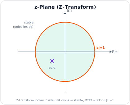
For a causal rational system, BIBO stability requires every pole to lie strictly inside the unit circle; the DTFT exists when the Z-transform ROC includes \(\lvert z\rvert=1\).
5. Laplace Transform¶
Likely Exam Question (past paper NTC 2079, 10 marks)
"Distinguish between Fourier transform, Laplace transform and z-transform. Find the Fourier transform of impulse function. List the properties of convolution."
Laplace Transform Definition¶
The bilateral Laplace transform, used for signal analysis and ROC arguments, is
Its ROC is the set of \(s\) values for which the integral converges. The factor \(e^{-\sigma t}\) allows the Laplace transform to represent a wider class of signals than the ordinary Fourier transform.
The unilateral Laplace transform, used to solve causal differential equations with initial conditions, is
These definitions must not be mixed: bilateral transforms carry ROC and two-sided-signal information, whereas unilateral transforms naturally incorporate initial conditions. For the right-sided signals in the following table, both produce the same algebraic expression.
Common Pairs¶
| \(x(t)\) | \(X(s)\) | ROC |
|---|---|---|
| \(\delta(t)\) | \(1\) | all \(s\) |
| \(u(t)\) | \(\frac{1}{s}\) | \(\Re(s) > 0\) |
| \(e^{-at}u(t)\) | \(\frac{1}{s+a}\) | \(\Re(s) > -a\) |
| \(\sin\omega_0t\,u(t)\) | \(\frac{\omega_0}{s^2+\omega_0^2}\) | \(\Re(s) > 0\) |
| \(\cos\omega_0t\,u(t)\) | \(\frac{s}{s^2+\omega_0^2}\) | \(\Re(s) > 0\) |
| \(t^nu(t)\) | \(\frac{n!}{s^{n+1}}\) | \(\Re(s) > 0\) |
Key Properties¶
The following differentiation and value-theorem formulas use the unilateral transform:
| Property | Result |
|---|---|
| Differentiation | \(\mathcal{L}_u\{x'(t)\} = sX_u(s) - x(0^-)\) |
| Integration | \(\mathcal{L}_u\{\int_0^t x(\tau)\,d\tau\} = \frac{X_u(s)}{s}\) |
| Convolution | \(x_1 * x_2 \leftrightarrow X_1(s)X_2(s)\) |
| Initial value | \(x(0^+) = \lim_{s\to\infty}sX_u(s)\) |
| Final value | \(\lim_{t\to\infty}x(t) = \lim_{s\to 0}sX_u(s)\), when its pole condition holds |
The final-value theorem is valid only when every pole of \(sX_u(s)\) lies strictly in the open left half-plane. Equivalently, \(X_u(s)\) may have a simple pole at the origin, while all its other poles must lie in the open left half-plane. The initial-value theorem also assumes that \(x(t)\) has no impulse at \(t=0\).
The Fourier transform is the bilateral Laplace transform evaluated on the imaginary axis,
but only when the bilateral Laplace ROC includes the complete \(j\omega\)-axis.
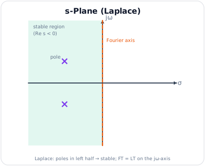
For a causal rational system, BIBO stability requires all poles to lie strictly in the open left half-plane (\(\Re s<0\)). The Fourier-transform relation additionally requires the bilateral ROC to contain the \(j\omega\)-axis.
6. Fourier vs Laplace vs Z — The Comparison (asked verbatim in 2079)¶
This section is the exact NTC 2079 composite [4 + 4 + 2 = 10]
Reproduce all three limbs together: (a) distinguish FT/LT/Z — the table below [4], (b) the Fourier transform of the impulse [4], (c) the properties of convolution [2].
| Feature | Fourier Transform | Laplace Transform | Z-Transform |
|---|---|---|---|
| Signal domain | Continuous-time | Continuous-time | Discrete-time |
| Variable | \(j\omega\) (imaginary axis only) | \(s = \sigma + j\omega\) (whole plane) | \(z = re^{j\Omega}\) (whole plane) |
| Definition | \(\int_{-\infty}^{\infty}x(t)e^{-j\omega t}dt\) | \(\int_{-\infty}^{\infty}x(t)e^{-st}dt\) | \(\sum_{n=-\infty}^{\infty}x[n]z^{-n}\) |
| Exists for | \(L^1\) is sufficient for the ordinary FT; distributions extend it further | Wider class through \(\sigma\) and the ROC | Wider class through radius \(r\) and the ROC |
| Initial conditions | Not handled | Handled naturally | Handled (unilateral ZT) |
| Main use | Spectrum/frequency content, filters, communication | Transient analysis, circuits, control systems, stability | Digital filters, DSP, discrete control |
| Stability test for causal rational systems | — | Poles strictly in the open LHP | Poles strictly inside the unit circle |
| Special case relation | Bilateral LT on \(s=j\omega\) | Generalizes the continuous-time FT | DTFT is ZT on \(z=e^{j\Omega}\) |
The Fourier Family at a Glance¶
The four Fourier representations are organised by whether the signal is continuous or discrete in time and periodic or aperiodic:
| Signal | Representation | Spectrum |
|---|---|---|
| Continuous-time, periodic | Fourier Series (FS) | discrete (lines), aperiodic |
| Continuous-time, aperiodic | Fourier Transform (FT) | continuous, aperiodic |
| Discrete-time, aperiodic | DTFT | continuous, periodic (\(2\pi\)) |
| Discrete-time, periodic / finite | DFT | discrete, periodic |
Laplace generalises the FT and Z generalises the DTFT by adding a real convergence factor (\(\sigma\) or radius \(r\)) — this is what enables ROC and transient/initial-condition analysis.
FT of the impulse function (also part of the 2079 question):
(by the sifting property — the impulse contains all frequencies equally).
Properties of convolution (third part of the 2079 question):
For \(y(t) = x(t) * h(t) = \int_{-\infty}^{\infty}x(\tau)h(t-\tau)d\tau\):
- Commutative: \(x * h = h * x\)
- Associative: \((x * h_1) * h_2 = x * (h_1 * h_2)\)
- Distributive: \(x * (h_1 + h_2) = x*h_1 + x*h_2\)
- Identity: \(x * \delta(t) = x(t)\); shift: \(x * \delta(t - t_0) = x(t - t_0)\)
- Time domain convolution ↔ frequency domain multiplication: \(x*h \leftrightarrow X(\omega)H(\omega)\)
- Width: duration of \(x*h\) = sum of durations; area of \(x*h\) = product of areas
7. Sampling: the Continuous-to-Discrete Bridge¶
Likely Exam Question (5 marks)
"State the sampling theorem. Explain aliasing and how the original signal is reconstructed."
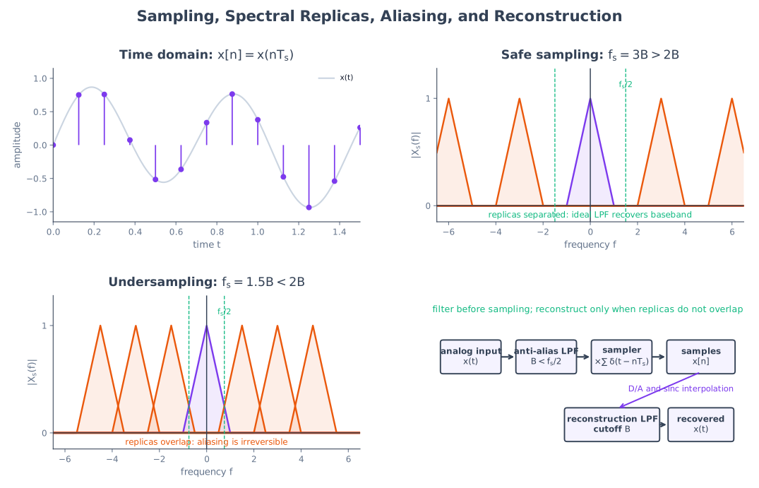
Sampling turns a continuous signal \(x(t)\) into the sequence \(x[n]=x(nT_s)\), taken every sampling interval \(T_s=1/f_s\). This is the step that connects the continuous transforms (FT, Laplace) to the discrete ones (DTFT, DFT, Z).
Sampling Theorem (Nyquist)¶
A signal band-limited to a maximum frequency \(f_m\) is fully recoverable from its samples only if
The minimum rate \(2f_m\) is the Nyquist rate; half the sampling rate, \(f_s/2\), is the Nyquist (folding) frequency.
Spectrum Replication and Aliasing¶
Ideal sampling replicates the signal spectrum, placing a copy centred at every integer multiple of \(f_s\). If \(f_s \ge 2f_m\) the copies stay separate and the baseband copy is intact. If \(f_s < 2f_m\) the copies overlap, so high frequencies fold back and masquerade as lower ones — this irreversible corruption is aliasing. It is prevented by an anti-aliasing low-pass filter that band-limits \(x(t)\) below \(f_s/2\) before sampling.
Reconstruction¶
An ideal low-pass filter of cutoff \(f_s/2\) keeps only the baseband copy and recovers \(x(t)\); in the time domain this is sinc interpolation (each sample is replaced by a scaled, shifted sinc). Practical systems use a sample-and-hold followed by a reconstruction (smoothing) filter.
Full treatment elsewhere
Sample-and-hold circuits, quantization and companding are covered in 5.4 Analog-to-Digital Conversion; the complete coding chain is in 5.7 PCM and ADPCM.
Key Exam Points - Transforms
- Fourier series is for periodic signals; Fourier transform is for aperiodic signals.
- Convolution in time becomes multiplication in frequency.
- Unit impulse has the sifting property; \(\mathcal{F}\{\delta(t)\} = 1\).
- Hilbert transform gives a \(90^\circ\) phase shift and forms analytic signal.
- Z transform is the main tool for discrete-time LTI systems and digital filters.
- Four Fourier representations: FS (CT periodic), FT (CT aperiodic), DTFT (DT aperiodic, \(2\pi\)-periodic), DFT (DT finite).
- Sampling theorem: \(f_s \ge 2f_m\); below the Nyquist rate, aliasing folds high frequencies down (use an anti-alias filter).
- Parseval preserves energy between time and frequency; duality pairs \(\delta\leftrightarrow 1\) with \(1\leftrightarrow 2\pi\delta\).
- The FT vs LT vs ZT comparison table + convolution properties were asked verbatim (NTC 2079) — reproduce §6 from memory.
Model Answer — Fourier, Laplace and z-Transform Comparison [4 marks]¶
Exam-ready answer
The three transforms express a signal as weighted complex exponentials, but they use different signal domains and convergence variables.
| Feature | Fourier transform | Bilateral Laplace transform | Bilateral z-transform |
|---|---|---|---|
| Signal | CT \(x(t)\) | CT \(x(t)\) | DT \(x[n]\) |
| Definition | \(X_F(\omega)=\int x(t)e^{-j\omega t}dt\) | \(X_L(s)=\int x(t)e^{-st}dt\) | \(X(z)=\sum x[n]z^{-n}\) |
| Variable | \(j\omega\) | \(s=\sigma+j\omega\) | \(z=re^{j\Omega}\) |
| Convergence | ordinary FT needs convergence on the frequency axis | vertical strip or half-plane ROC | annular ROC |
| Main use | spectrum and frequency response | CT transients, differential equations and stability | DT systems, difference equations and digital filters |
The Fourier transform is the Laplace transform on \(s=j\omega\) only when the bilateral Laplace ROC contains the complete imaginary axis. Likewise, the DTFT is \(X(z)\) on \(z=e^{j\Omega}\) only when the z-transform ROC contains the unit circle. For causal rational systems, stability requires poles strictly in the open left half-plane in the \(s\)-plane or strictly inside the unit circle in the \(z\)-plane.
Laplace and z transforms also retain ROC information, so the same rational expression can represent different right- or left-sided signals. Unilateral versions are used when initial conditions must be included. Thus FT is primarily spectral, LT generalises CT Fourier analysis by exponential weighting, and z-transform is the corresponding generalisation for sequences.
Practice target: 7 minutes; reproduce the definition/domain/ROC table and state both special-case relations with their convergence conditions.
Model Answer — Fourier Transform of the Unit Impulse [4 marks]¶
Exam-ready answer
With the angular-frequency Fourier-transform convention
put \(x(t)=\delta(t)\). The sifting property \(\int f(t)\delta(t-t_0)dt=f(t_0)\) gives
More generally,
The magnitude is \(|A|\) at every angular frequency and the delay contributes linear phase \(-\omega t_0\). Therefore an ideal impulse has a flat, infinitely wide spectrum: it contains all frequencies with equal magnitude. If it is applied to an LTI system, \(Y(\omega)=1\cdot H(\omega)=H(\omega)\), so the measured output is the impulse response and its transform is the system frequency response.
As a consistency check, inverse transforming \(1\) gives
in the distribution sense. The impulse is not an ordinary finite-energy pulse; the result relies on the generalized-function sifting definition.
Practice target: 5 minutes; write the convention, one-line sifting derivation, shifted result and flat-spectrum interpretation.
Model Answer — Fourier-Transform Properties and Proofs [5–10 marks]¶
5-mark answer and 10-mark extension
For 5 marks — write this¶
For the transform pair
the important properties are:
| Time-domain operation | Frequency-domain result |
|---|---|
| \(a x_1(t)+b x_2(t)\) | \(aX_1(\omega)+bX_2(\omega)\) |
| \(x(t-t_0)\) | \(e^{-j\omega t_0}X(\omega)\) |
| \(e^{j\omega_0t}x(t)\) | \(X(\omega-\omega_0)\) |
| \(x(at)\) | \(\lvert a\rvert^{-1}X(\omega/a)\) |
| \(dx/dt\) | \(j\omega X(\omega)\) |
| \(x*h\) | \(XH\) |
Parseval’s theorem is \(\int|x(t)|^2dt=(2\pi)^{-1}\int|X(\omega)|^2d\omega\). If \(x(t)\) is real, \(X(-\omega)=X^*(\omega)\), so magnitude is even and phase is odd. Absolute integrability of \(x\) is a sufficient condition for an ordinary FT; energy signals also possess an \(L^2\) transform, and impulses are handled as distributions.
Add for a 10-mark variant¶
Time-shift proof. Put \(v=t-t_0\):
A delay changes phase but not magnitude.
Differentiation proof. Assuming \(x(t)\) decays sufficiently for the boundary term to vanish, integration by parts gives
Convolution proof. If \(y(t)=\int x(\tau)h(t-\tau)d\tau\) and the integrals may be interchanged, then with \(v=t-\tau\),
The companion multiplication property is \(x(t)g(t)\leftrightarrow(2\pi)^{-1}X*G\). Duality states that if \(x(t)\leftrightarrow X(\omega)\), then \(X(t)\leftrightarrow2\pi x(-\omega)\). For example, duality converts \(\delta(t)\leftrightarrow1\) into \(1\leftrightarrow2\pi\delta(\omega)\).
Application: since \(e^{-at}u(t)\leftrightarrow1/(a+j\omega)\) for \(a>0\), delaying it by \(t_0\) gives
This single result demonstrates transform existence, time shift, magnitude invariance under delay and linear phase.
Practice target: 9 minutes for the property table or 18 minutes with three proofs; state assumptions before interchanging integrals or discarding boundary terms.
Model Answer — Hilbert Transform and SSB Generation [5 marks]¶
Exam-ready answer
The Hilbert transform of \(x(t)\) is convolution with \(1/(\pi t)\), interpreted as a Cauchy principal value:
Its frequency response is
Thus it leaves magnitude unchanged, shifts positive-frequency components by \(-90^\circ\), and shifts negative-frequency components by \(+90^\circ\). For example, under this convention \(\mathcal H\{\cos\omega_mt\}=\sin\omega_mt\). The analytic signal
has spectrum \(2X(\omega)\) for \(\omega>0\), zero for \(\omega<0\), with the DC value unchanged; this assumes real \(x(t)\).
In the phase-shift method of SSB generation, \(m(t)\) and \(\hat m(t)\) modulate quadrature carriers:
For \(m(t)=\cos\omega_mt\), substitute \(\hat m(t)=\sin\omega_mt\) and use angle identities:
One sideband reinforces and the other cancels because both message paths and both carrier paths are in exact quadrature. Practical cancellation is limited by Hilbert-network amplitude and phase errors. SSB occupies only message bandwidth \(B_m\), half the bandwidth of conventional AM, and suppressing the carrier avoids wasted carrier power.
Practice target: 9 minutes; state the PV definition, frequency multiplier, analytic signal and prove cancellation with a single-tone message.
Model Answer — z-Transform Properties and Standard Sequence [5 marks]¶
Exam-ready answer
The bilateral z-transform of a DT sequence is
The region of convergence (ROC) is the annulus in the z-plane where this sum converges. The algebraic expression without its ROC is incomplete because right- and left-sided sequences can have the same rational expression.
| Property | z-domain result |
|---|---|
| \(a x[n]+b y[n]\) | \(aX(z)+bY(z)\) |
| \(x[n-n_0]\) | \(z^{-n_0}X(z)\) |
| \(x[n]*y[n]\) | \(X(z)Y(z)\) |
| \(n x[n]\) | \(-z\,dX(z)/dz\) |
| \(x[-n]\) | \(X(z^{-1})\) |
For a causal sequence, \(x[0]=\lim_{z\to\infty}X(z)\). The final-value theorem is \(\lim_{n\to\infty}x[n]=\lim_{z\to1}(1-z^{-1})X(z)\) only when its pole condition is satisfied: after removing a possible simple pole at \(z=1\), all poles must be strictly inside the unit circle.
Standard derivation: for \(x[n]=a^nu[n]\),
and the geometric series requires \(|az^{-1}|<1\), hence
For \(a=1/2\), the pole is at \(z=0.5\) and the causal ROC includes the unit circle, so the DTFT exists and the corresponding causal LTI impulse response is stable. In general, a causal rational system has ROC outside its outermost pole; it is BIBO stable when the ROC includes \(|z|=1\), so causal and stable implies all poles strictly inside the unit circle.
Practice target: 9 minutes; always write the ROC beside the transform and state the pole condition before using a value theorem.
Model Answer — Fourier Series, FT, DTFT and DFT [5 marks]¶
Exam-ready answer
The four Fourier representations are selected by whether time is continuous or discrete and whether the signal is periodic or aperiodic.
| Signal class | Representation and definition | Spectrum |
|---|---|---|
| CT periodic, period \(T_0\) | FS: \(x(t)=\sum_{k=-\infty}^{\infty}C_ke^{jk\omega_0t}\), \(C_k=T_0^{-1}\int_{T_0}x(t)e^{-jk\omega_0t}dt\) | discrete lines at \(k\omega_0\) |
| CT aperiodic | FT: \(X(\omega)=\int_{-\infty}^{\infty}x(t)e^{-j\omega t}dt\) | continuous, generally aperiodic |
| DT aperiodic | DTFT: \(X(e^{j\Omega})=\sum_{n=-\infty}^{\infty}x[n]e^{-j\Omega n}\) | continuous and \(2\pi\)-periodic |
| finite \(N\)-sample record | DFT: \(X[k]=\sum_{n=0}^{N-1}x[n]e^{-j2\pi kn/N}\) | \(N\) discrete, periodic bins |
The inverse DFT is \(x[n]=N^{-1}\sum_{k=0}^{N-1}X[k]e^{j2\pi kn/N}\). It treats both \(x[n]\) and \(X[k]\) as one period of periodic sequences. The DFT samples the DTFT at \(\Omega_k=2\pi k/N\) when the finite record is taken as one period; it is not a separate physical spectrum.
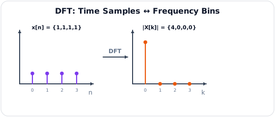
The line spectrum of FS occurs because a periodic signal contains only integer harmonics of \(\omega_0=2\pi/T_0\). Letting the period tend to infinity makes line spacing tend to zero and leads to the continuous FT. Sampling time makes frequency periodic, explaining DTFT periodicity; sampling one period of the DTFT gives DFT bins.
Convergence conditions must be stated: piecewise smooth periodic signals satisfying Dirichlet conditions possess an FS (with midpoint convergence at jumps); absolute summability \(\sum|x[n]|<\infty\) is sufficient for a DTFT. Laplace generalises the CT FT, and z-transform generalises the DTFT; the FT or DTFT is obtained only when the relevant ROC includes the imaginary axis or unit circle.
Practice target: 10 minutes; draw the two-by-two classification table and write one defining analysis equation plus the spectrum type for every representation.
Model Answer — Sampling Theorem, Aliasing and Reconstruction [5 marks]¶
Exam-ready answer
Let a CT signal \(x(t)\) be band-limited so that \(X(f)=0\) for \(|f|>f_m\). Uniform ideal sampling every \(T_s\) seconds gives \(x[n]=x(nT_s)\) and \(f_s=1/T_s\). The sampling theorem states that exact recovery is possible when
with \(2f_m\) called the Nyquist rate and \(f_s/2\) the Nyquist frequency. Equality is an ideal limiting case and is avoided in practice because realizable filters need a transition band.
Represent sampling by the impulse train \(p(t)=\sum_n\delta(t-nT_s)\). Since \(x_s(t)=x(t)p(t)\),
Thus sampling creates spectral replicas spaced by \(f_s\). If \(f_s>2f_m\), adjacent copies do not overlap. If \(f_s<2f_m\), they overlap and different analog frequencies produce identical samples; this irreversible folding is aliasing.
An input sinusoid at frequency \(f_0\) aliases to \(|f_0-kf_s|\) chosen in \([0,f_s/2]\). For example, sampling \(900\) Hz at \(f_s=1\) kHz produces samples indistinguishable from a \(|900-1000|=\boxed{100\text{ Hz}}\) sinusoid.
Before the sampler, an analog anti-alias low-pass filter restricts the input below \(f_s/2\). After sampling, an ideal reconstruction LPF selects the baseband replica. Equivalently, ideal time-domain reconstruction is sinc interpolation:
for the normalized sinc \(\operatorname{sinc}(v)=\sin(\pi v)/(\pi v)\). Practical converters use a sample-and-hold and a reconstruction filter, with sampling rate chosen above Nyquist to allow nonideal filter roll-off.
Practice target: 9 minutes; state the band-limit assumption, draw spectral replicas, calculate one alias and name both anti-alias and reconstruction filters.