Frequency Response Method
Possible Exam Questions
Exam Questions and Answer Map
Questions labelled [PYQ paper/year] are observed past questions; those labelled [likely] are pattern-based predictions. For each one, rehearse the answer plan closed-book, then use the links to verify the full answer in this chapter.
-
Define frequency response; state its advantages as an analysis method. [5] — [likely]
-
Answer plan: Define frequency response as steady-state output to sinusoidal input → write \(G(j\omega)\) in magnitude-phase form → list advantages (experimental, high-order systems, compensator design, noise analysis, easy Bode asymptotes).
-
Model answer: Frequency-response definition and advantages
-
Define gain margin and phase margin; how do they indicate relative stability? [5] — [likely]
-
Answer plan: Define gain crossover and phase crossover frequencies → define GM = \(-20\log|G(j\omega_{pc})|\) dB → define PM = \(180° + \angle G(j\omega_{gc})\) → state that positive GM and PM indicate stability → relate larger margins to more robust system.
-
Model answer: Gain margin, phase margin, and relative stability
-
Sketch and explain the Bode plot; state its construction rules. [10] — [likely]
-
Answer plan: Define Bode plot (magnitude in dB and phase in degrees vs log frequency) → list standard factors (constant, integrator, first-order pole/zero, second-order) → state asymptotic slopes → explain corner frequency corrections → sketch a sample composite plot.
-
Model answer: Bode-plot construction, second-order response, and compensation
-
Explain the Nyquist/polar plot and the Nyquist stability criterion. [5–10] — [likely]
-
Answer plan: Define polar plot (magnitude and phase in complex plane) → state Nyquist criterion \(Z = N + P\) → define encirclements of \(-1+j0\) → for open-loop stable system: no encirclement means closed-loop stable → explain practical interpretation.
- Model answer: Polar plot and Nyquist stability criterion
Syllabus Focus
- Frequency response method
- Sinusoidal steady-state response
- Bode plot analysis
- Polar and Nyquist plots
- Gain margin and phase margin
- Bandwidth, resonance, and relative stability
- Frequency-domain compensation basics
1. Introduction to Frequency Response
Likely Exam Question (5 marks)
"Define frequency response. State the advantages of frequency-response analysis in control systems."
The frequency response of a system is the steady-state response of the system to a sinusoidal input as the input frequency is varied.
For input:
the steady-state output of a stable linear time-invariant system is:
The output has the same frequency as input, but different amplitude and phase.
Frequency Response from Transfer Function
Given transfer function \(G(s)\), substitute:
Then:
where:
- \(|G(j\omega)|\) = magnitude ratio
- \(\angle G(j\omega)\) = phase shift
If input amplitude is \(A\), output amplitude is:
and phase shift is:
Advantages
- Can be obtained experimentally without deriving full mathematical model.
- Useful for stability analysis of high-order systems.
- Gives gain margin and phase margin directly.
- Helps design compensators and filters.
- Useful for noise and bandwidth analysis.
- Bode plots are easy to sketch using asymptotic rules.
2. Important Frequency-Domain Quantities
Likely Exam Question (5 marks)
"Define gain crossover frequency, phase crossover frequency, gain margin, and phase margin."
Magnitude in Decibels
Magnitude is usually expressed in decibels:
If magnitude is power ratio:
Gain Crossover Frequency
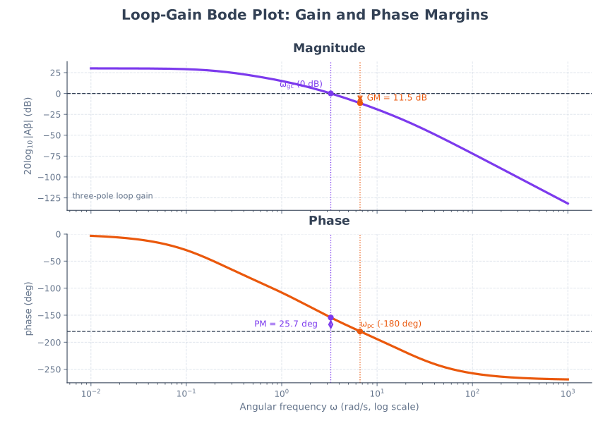
Gain crossover frequency \(\omega_{gc}\) is the frequency at which magnitude is unity or 0 dB.
or:
Phase Crossover Frequency
Phase crossover frequency \(\omega_{pc}\) is the frequency at which phase angle is \(-180^\circ\).
Gain Margin
Gain margin is the factor by which loop gain can be increased before the system becomes unstable.
At phase crossover frequency:
In decibels:
Phase Margin
Phase margin is the additional phase lag required at gain crossover frequency to make the system marginally stable.
Stability Interpretation
For a stable open-loop minimum-phase system:
| Margin | Meaning |
|---|---|
| \(GM>1\) or \(GM_{dB}>0\) | Stable gain margin |
| \(GM=1\) or \(GM_{dB}=0\) | Marginal stability |
| \(GM<1\) or \(GM_{dB}<0\) | Unstable closed-loop system |
| \(PM>0\) | Stable phase margin |
| \(PM=0\) | Marginal stability |
| \(PM<0\) | Unstable closed-loop system |
Practical control systems often target:
and:
3. Bode Plot
Likely Exam Question (10 marks)
"Draw the Bode plot of a given transfer function and determine gain margin and phase margin."
A Bode plot consists of two plots against logarithmic frequency:
- Magnitude plot: \(20\log_{10}|G(j\omega)|\) vs \(\log\omega\)
- Phase plot: \(\angle G(j\omega)\) vs \(\log\omega\)
Advantages of Bode Plot
- Multiplication of factors becomes addition in dB.
- Wide frequency range can be shown compactly.
- Simple straight-line asymptotes can approximate response.
- Gain margin and phase margin are easily read.
- Useful for compensator design.
Standard Factors
| Factor | Magnitude Slope | Phase Contribution |
|---|---|---|
| Constant \(K\) | \(20\log K\) dB | \(0^\circ\) if \(K>0\), \(180^\circ\) if \(K<0\) |
| Pole at origin \(1/s\) | \(-20\) dB/dec | \(-90^\circ\) |
| Zero at origin \(s\) | \(+20\) dB/dec | \(+90^\circ\) |
| First-order pole \(1/(1+sT)\) | 0 then \(-20\) dB/dec after \(1/T\) | 0 to \(-90^\circ\) |
| First-order zero \((1+sT)\) | 0 then \(+20\) dB/dec after \(1/T\) | 0 to \(+90^\circ\) |
| Second-order pole | 0 then \(-40\) dB/dec after \(\omega_n\) | 0 to \(-180^\circ\) |
| Second-order zero | 0 then \(+40\) dB/dec after \(\omega_n\) | 0 to \(+180^\circ\) |
Frequency Units
A decade is a 10:1 frequency ratio.
An octave is a 2:1 frequency ratio.
Slope conversions:
4. Bode Plot Construction Rules
Likely Exam Question (10 marks)
"Explain the rules for constructing magnitude and phase Bode plots."
Step 1 - Put Transfer Function in Standard Form
Write:
or for second-order factors:
Step 2 - Identify Corner Frequencies
For factor \((1+sT)\):
For second-order factor:
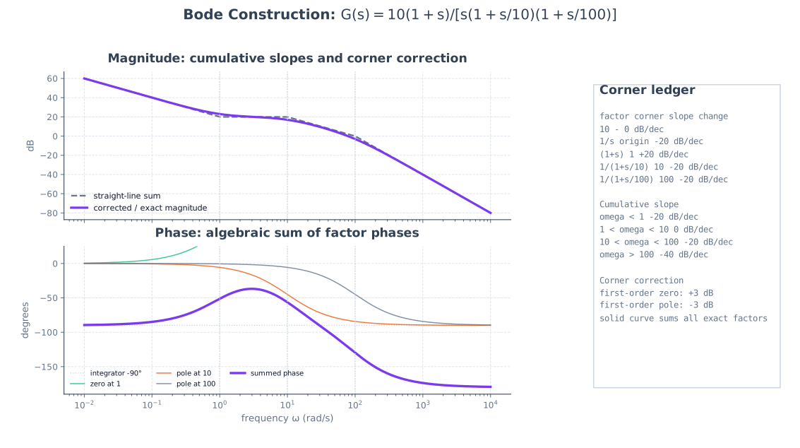
Step 3 - Draw Magnitude Asymptotes
- Start with constant gain \(20\log_{10}K\).
- Add \(+20\) dB/dec for each zero at origin.
- Add \(-20\) dB/dec for each pole at origin.
- At each first-order zero corner, increase slope by \(+20\) dB/dec.
- At each first-order pole corner, decrease slope by \(-20\) dB/dec.
- At each second-order zero, increase slope by \(+40\) dB/dec.
- At each second-order pole, decrease slope by \(-40\) dB/dec.
Step 4 - Apply Corrections if Needed
At first-order corner frequency:
- Actual magnitude of zero is \(+3\) dB above asymptote.
- Actual magnitude of pole is \(-3\) dB below asymptote.
For second-order factors, resonant peak depends strongly on damping ratio \(\zeta\).
Step 5 - Draw Phase Plot
Approximate phase change for a first-order pole or zero occurs from one decade below to one decade above corner frequency.
For first-order pole \(1/(1+sT)\):
For first-order zero \((1+sT)\):
Approximate values:
| Frequency | First-Order Pole Phase | First-Order Zero Phase |
|---|---|---|
| \(0.1\omega_c\) | \(0^\circ\) | \(0^\circ\) |
| \(\omega_c\) | \(-45^\circ\) | \(+45^\circ\) |
| \(10\omega_c\) | \(-90^\circ\) | \(+90^\circ\) |
5. Frequency Response of Standard Factors
Constant Gain
For \(G(s)=K\):
Phase is \(0^\circ\) for positive \(K\).
Integrator
For:
Magnitude:
Magnitude in dB:
Phase:
First-Order Pole
For:
Magnitude:
Phase:
At corner frequency \(\omega_c=1/T\):
First-Order Zero
For:
Magnitude:
Phase:
6. Second-Order Frequency Response
Likely Exam Question (10 marks)
"Derive resonant peak, resonant frequency, and bandwidth of a standard second-order system."
Standard second-order closed-loop transfer function:
Frequency response:
Magnitude:
Phase:
Resonant Peak
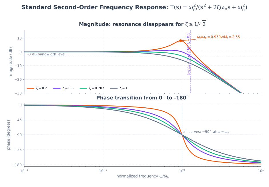
Resonant peak \(M_r\) is maximum value of \(|T(j\omega)|\).
For \(0<\zeta<1/\sqrt2\):
If \(\zeta\ge1/\sqrt2\), there is no resonant peak.
Resonant Frequency
Frequency at which resonant peak occurs:
valid for \(0<\zeta<1/\sqrt2\).
Bandwidth
Bandwidth is the frequency at which magnitude drops to \(1/\sqrt2\) of low-frequency value, or -3 dB point.
For standard second-order system:
Interpretation
- Higher bandwidth means faster time response.
- Higher resonant peak generally means larger overshoot.
- Larger damping ratio reduces resonance and overshoot.
7. Polar Plot
Likely Exam Question (5 marks)
"What is a polar plot? How is it used in frequency-response analysis?"
A polar plot is a plot of \(G(j\omega)\) in the complex plane as frequency varies from \(0\) to \(\infty\).
Each point has:
- Radius = \(|G(j\omega)|\)
- Angle = \(\angle G(j\omega)\)
Procedure
- Substitute \(s=j\omega\) in transfer function.
- Find magnitude and phase at key frequencies.
- Plot points in complex plane.
- Join points smoothly as \(\omega\) increases from \(0\) to \(\infty\).
Important Points
- Starting point: value at \(\omega=0\).
- Ending point: value as \(\omega\to\infty\).
- Intersections with real and imaginary axes help determine margins.
- Polar plot is the basis for Nyquist stability criterion.
8. Nyquist Stability Criterion
Likely Exam Question (10 marks)
"State Nyquist stability criterion and explain how it determines closed-loop stability."
Nyquist criterion determines closed-loop stability from the frequency response of open-loop transfer function \(G(s)H(s)\).
Closed-loop characteristic equation:
Critical point:
Nyquist Criterion
Let:
- \(P\) = number of open-loop poles of \(G(s)H(s)\) in right half-plane
- \(N\) = net number of clockwise encirclements of \(-1+j0\) by Nyquist plot
- \(Z\) = number of closed-loop poles in right half-plane
Then:
For closed-loop stability:
Therefore:
depending on sign convention for clockwise encirclements.
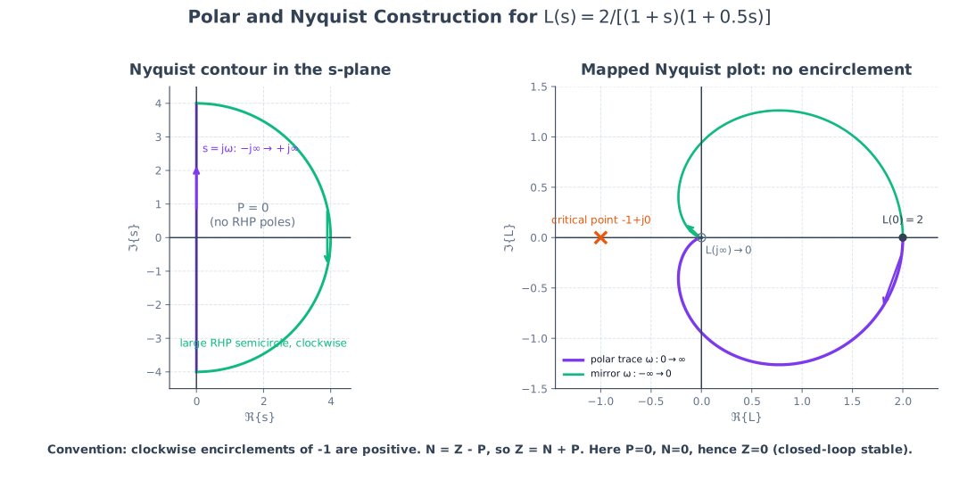
If the open-loop system is stable, \(P=0\), then closed-loop system is stable if the Nyquist plot does not encircle \(-1+j0\).
Practical Interpretation
For open-loop stable systems:
- If Nyquist plot does not encircle \(-1\), closed-loop system is stable.
- If Nyquist plot passes through \(-1\), system is marginally stable.
- If Nyquist plot encircles \(-1\), closed-loop system is unstable.
9. Gain Margin and Phase Margin from Bode Plot
Likely Exam Question (10 marks)
"Find gain margin and phase margin from a Bode plot. Comment on stability."
Finding Phase Margin
- Find gain crossover frequency \(\omega_{gc}\) where magnitude crosses 0 dB.
- Read phase angle at \(\omega_{gc}\).
- Compute:
where \(\phi_{gc}=\angle G(j\omega_{gc})H(j\omega_{gc})\).
Finding Gain Margin
- Find phase crossover frequency \(\omega_{pc}\) where phase is \(-180^\circ\).
- Read magnitude at \(\omega_{pc}\) in dB.
- Compute:
If magnitude at phase crossover is \(-10\) dB, gain margin is \(+10\) dB.
Relationship to Time Response
| Margin | Time-Domain Meaning |
|---|---|
| Small PM | More oscillatory, larger overshoot |
| Large PM | Better damping, slower response if too large |
| Low GM | Gain changes can destabilize system |
| High GM | More robust to gain variation |
Approximate relation for many second-order-like systems:
This is only an approximation.
10. Relative Stability in Frequency Domain
Likely Exam Question (5 marks)
"Explain relative stability using frequency-response measures."
Relative stability describes how far the system is from instability.
Frequency-domain measures:
| Measure | Meaning |
|---|---|
| Gain margin | Gain increase allowed before instability |
| Phase margin | Additional phase lag allowed before instability |
| Resonant peak \(M_r\) | Indicates oscillatory tendency |
| Bandwidth \(\omega_b\) | Indicates speed of response |
| Crossover frequency | Roughly related to response speed |
Bandwidth and Speed
Higher bandwidth usually means faster response, but also more noise sensitivity.
Resonant Peak and Overshoot
Larger resonant peak usually means larger transient overshoot and poorer damping.
Design Trade-Off
Control design balances:
- Fast response
- Low overshoot
- Good stability margins
- Low steady-state error
- Noise rejection
- Actuator limitations
11. Frequency-Domain Compensation
Likely Exam Question (5 marks)
"Compare lag, lead, and lag-lead compensators in frequency-response design."
Compensation modifies frequency response to satisfy performance requirements.
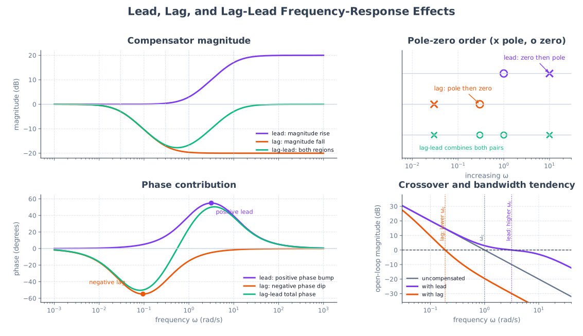
Lead Compensator
Transfer function:
Effects:
- Adds positive phase lead.
- Increases phase margin.
- Increases bandwidth.
- Improves transient response.
Lag Compensator
Transfer function:
Effects:
- Improves steady-state accuracy.
- Increases low-frequency gain.
- Usually decreases bandwidth.
- Has small negative phase contribution.
Lag-Lead Compensator
Combines lag and lead actions.
Effects:
- Improves steady-state accuracy.
- Improves transient response.
- Improves stability margin.
PID in Frequency Domain
PID controller:
Effects:
| Action | Frequency-Domain Effect | Main Benefit |
|---|---|---|
| P | Raises gain | Speeds response, reduces error |
| I | Raises low-frequency gain | Eliminates steady-state error |
| D | Adds phase lead | Improves damping and stability |
12. Solved Examples
Example 1 - Frequency Response of First-Order System
Q. For \(G(s)=\frac{10}{s+10}\), find magnitude and phase at \(\omega=10\,\text{rad/s}\).
Solution:
At \(\omega=10\):
Magnitude:
Magnitude in dB:
Phase:
Example 2 - Gain and Phase Margin
Q. At phase crossover frequency, \(|G(j\omega_{pc})H(j\omega_{pc})|=0.25\). At gain crossover frequency, phase is \(-135^\circ\). Find gain margin and phase margin.
Solution:
Gain margin:
In dB:
Phase margin:
The margins are positive, so the system is stable with reasonable relative stability.
Example 3 - Bode Magnitude Slopes
Q. Sketch asymptotic magnitude slope for:
Solution:
Factors:
- Gain \(100\) gives \(40\) dB.
- Pole at origin gives initial slope \(-20\) dB/dec.
- Pole at \(10\) rad/s decreases slope by \(-20\) dB/dec.
- Pole at \(100\) rad/s decreases slope by another \(-20\) dB/dec.
Slopes:
| Frequency Range | Slope |
|---|---|
| \(\omega<10\) | \(-20\) dB/dec |
| \(10<\omega<100\) | \(-40\) dB/dec |
| \(\omega>100\) | \(-60\) dB/dec |
Example 4 - Resonant Peak
Q. A second-order system has \(\zeta=0.4\) and \(\omega_n=20\,\text{rad/s}\). Find resonant frequency and resonant peak.
Solution:
Since \(\zeta<1/\sqrt2\), resonance exists.
In dB:
Example 5 - Nyquist Stability
Q. An open-loop stable system has Nyquist plot that does not encircle \(-1+j0\). Is the closed-loop system stable?
Solution:
Open-loop stable means:
No encirclement means:
Nyquist criterion:
No closed-loop poles in right half-plane, so:
13. Quick Revision Table
| Topic | Key Result |
|---|---|
| Frequency response | Evaluate \(G(s)\) at \(s=j\omega\) |
| Magnitude in dB | \(20\log_{10}\lvert G(j\omega)\rvert\) |
| Gain crossover frequency | \(\lvert G(j\omega_{gc})H(j\omega_{gc})\rvert=1\) |
| Phase crossover frequency | \(\angle G(j\omega_{pc})H(j\omega_{pc})=-180^\circ\) |
| Gain margin | \(GM=1/\lvert G(j\omega_{pc})H(j\omega_{pc})\rvert\) |
| Gain margin in dB | \(GM_{dB}=-20\log_{10}\lvert G(j\omega_{pc})H(j\omega_{pc})\rvert\) |
| Phase margin | \(PM=180^\circ+\angle G(j\omega_{gc})H(j\omega_{gc})\) |
| First-order pole phase | \(-\tan^{-1}(\omega T)\) |
| First-order zero phase | \(+\tan^{-1}(\omega T)\) |
| Integrator slope | \(-20\) dB/dec, phase \(-90^\circ\) |
| Differentiator slope | \(+20\) dB/dec, phase \(+90^\circ\) |
| Resonant peak | \(M_r=1/[2\zeta\sqrt{1-\zeta^2}]\) |
| Resonant frequency | \(\omega_r=\omega_n\sqrt{1-2\zeta^2}\) |
| Nyquist criterion | \(Z=N+P\) |
| Critical point | \(-1+j0\) |
Key Exam Points - Frequency Response
- Substitute \(s=j\omega\) to get frequency response.
- Bode magnitude slopes change by \(20\) dB/dec for each first-order pole or zero.
- Positive gain margin and phase margin indicate stable relative behavior for minimum-phase open-loop stable systems.
- Nyquist stability depends on encirclements of the critical point \(-1+j0\).
- Higher bandwidth gives faster response but usually increases noise sensitivity.
Model Answer — Frequency-Response Definition and Advantages [5 marks]
Exam-ready answer
The frequency response of a stable LTI system is its sinusoidal steady-state gain and phase shift as angular frequency \(\omega\) is varied. Adopt the \(e^{j\omega t}\) convention and a positive output measured in the declared physical direction. If
then, after transients decay,
This follows because \(e^{j\omega t}\) is an eigenfunction of an LTI system: substituting \(s=j\omega\) into its transfer function gives
Here \(\omega\) is rad/s, \(f=\omega/(2\pi)\) is hertz, magnitude has the output/input unit ratio, and phase is in degrees or radians. Magnitude is often expressed as \(20\log_{10}M\) dB.
Advantages of frequency-response analysis:
- \(G(j\omega)\) can be measured by applying sinusoids even when a detailed differential-equation model is unavailable.
- Bode logarithms turn products into sums and make high-order pole/zero effects easy to sketch.
- Gain margin, phase margin and Nyquist encirclements assess absolute and relative closed-loop stability from the open-loop response.
- Bandwidth, resonance and roll-off connect speed, damping and noise rejection.
- Lead, lag and PID compensators can be designed by shaping gain and phase over selected frequency bands.
- Parasitic high-frequency dynamics, resonances and sensor noise are often clearer than in a time plot.
Worked check: for \(G(s)=1/(1+s\tau)\) with \(\tau>0\) s,
At \(\omega=1/\tau\), \(M=1/\sqrt2=-3.01\) dB and \(\phi=-45^\circ\), identifying the bandwidth of this first-order low-pass system.
The method describes steady state, not startup transients, and an unstable system does not physically settle even though its formal \(G(j\omega)\) can be evaluated. Nonlinear systems depend on input amplitude, and delays/unmodeled modes can invalidate a measured low-frequency model. Frequency and time responses are complementary rather than competing methods.
Practice target: 9 minutes; derive the sinusoidal output from \(G(j\omega)\), list six advantages, and verify the first-order corner.
Model Answer — Gain Margin, Phase Margin, and Relative Stability [5 marks]
Exam-ready answer
For a negative-feedback system, define the open-loop transfer \(L(s)=G(s)H(s)\) and characteristic equation \(1+L(s)=0\). Use the \(e^{j\omega t}\) convention and unwrap phase continuously near \(-180^\circ\).
The gain crossover frequency \(\omega_{gc}\) in rad/s satisfies
The additional phase lag required there to reach the critical angle \(-180^\circ\) is the phase margin:
The phase crossover frequency \(\omega_{pc}\) satisfies
The multiplicative gain increase that would move that point to \(-1+j0\) is the gain margin:
For the common case of an open-loop stable, minimum-phase system with one relevant crossover, \(GM>1\) (\(GM_{dB}>0\)) and \(PM>0\) indicate closed-loop stability. Larger positive margins usually mean better tolerance to gain variation, delay and modeling error; very small margins imply oscillatory response and high resonant peak. Excessively large margins may accompany low crossover frequency and sluggish response, so margins are design tradeoffs, not quantities to maximize without limit.
Worked check: suppose the phase at \(\omega_{gc}\) is \(-135^\circ\) and magnitude at \(\omega_{pc}\) is \(-8\) dB. Then
Thus gain can increase by a factor about 2.51 before the simple crossover model reaches marginal stability. With multiple crossovers, RHP open-loop poles, nonminimum-phase zeros or delay, merely seeing positive-looking margins can be misleading; use the full Nyquist criterion and report the most restrictive margins. Undefined crossover means an infinite or undefined margin according to the actual curve, not automatically a safe design.
Practice target: 9 minutes; mark each margin at its opposite crossover and include both dB and multiplicative gain in the numerical check.
Model Answer — Bode-Plot Construction, Second-Order Response, and Compensation [10 marks]
Exam-ready answer
A Bode plot consists of \(20\log_{10}|G(j\omega)|\) in dB and \(\angle G(j\omega)\) in degrees versus logarithmic angular frequency \(\omega\) in rad/s. With \(e^{j\omega t}\), positive phase means output leads input. First factor the transfer function into normalized real poles, zeros, origin factors and quadratic factors; magnitudes in dB and phases then add.
For
use these rules:
| Factor | Magnitude asymptote | Phase |
|---|---|---|
| \(K>0\) | \(20\log_{10}K\) dB | \(0^\circ\) |
| \(s\) / \(1/s\) | \(+20/-20\) dB/dec from origin | \(+90^\circ/-90^\circ\) |
| \(1+j\omega/\omega_c\) | slope increases \(20\) dB/dec after \(\omega_c\) | \(+\tan^{-1}(\omega/\omega_c)\) |
| \(1/(1+j\omega/\omega_c)\) | slope decreases \(20\) dB/dec after \(\omega_c\) | \(-\tan^{-1}(\omega/\omega_c)\) |
A first-order zero is \(+3.01\) dB and a pole is \(-3.01\) dB relative to its intersecting asymptotes at \(\omega_c\). Approximate phase changes from one decade below to one decade above the corner and is \(\pm45^\circ\) at the corner. Repeated factors multiply slope and phase contributions.
Construction procedure: normalize and list every corner; calculate the initial dB level and slope; change cumulative slope at each corner; apply exact corner corrections where accuracy is required; add all factor phases; finally mark \(\omega_{gc}\), \(\omega_{pc}\), margins and bandwidth.
Worked check: for
the initial slope is \(-20\) dB/dec, changing to \(-40\) at \(10\) rad/s and \(-60\) at \(100\) rad/s. Exact phase is
At \(\omega=10\) rad/s, magnitude is
and phase is approximately \(-140.7^\circ\), checking the first corner correction.
For the standard second-order low-pass factor
let \(r=\omega/\omega_n\). Then
Its high-frequency slope is \(-40\) dB/dec and phase changes from \(0^\circ\) toward \(-180^\circ\). If \(0<\zeta<1/\sqrt2\), resonance occurs at \(\omega_r=\omega_n\sqrt{1-2\zeta^2}\) with \(M_r=1/[2\zeta\sqrt{1-\zeta^2}]\); greater damping removes the peak.
Compensation: a lead network
places its zero below its pole and contributes positive phase, usually increasing phase margin, crossover and bandwidth. A lag network
places its pole below its zero, raises low-frequency gain relative to high-frequency gain after scaling, improves steady-state accuracy, adds negative phase and usually lowers bandwidth. Lag-lead combines both goals.
Asymptotes are design approximations; exact curves are needed near lightly damped resonances and crossover. High bandwidth speeds response but passes more noise and may expose unmodeled poles. Bode design therefore requires a proper loop model and final Nyquist/time-domain verification.
Practice target: 20 minutes; create a corner/slope ledger, calculate one exact point, and reserve the final section for quadratic response and lead-lag tradeoffs.
Model Answer — Polar Plot and Nyquist Stability Criterion [10 marks]
Exam-ready answer
Let \(L(s)=G(s)H(s)\) be the open-loop transfer of a negative-feedback system, so closed-loop poles satisfy
A polar plot traces the complex number \(L(j\omega)=|L|\angle L\) as positive frequency varies from \(0\) to \(\infty\): radius is magnitude and angle is phase. A Nyquist plot is more complete: it maps the entire Nyquist contour that encloses the right half of the \(s\)-plane, including positive and negative frequencies, the infinite semicircle, and small indentations around any imaginary-axis poles. For real-coefficient systems the negative-frequency branch is the complex conjugate of the positive-frequency polar trace.
The critical point is \(-1+j0\) because \(1+L=0\) there. Declare the sign convention before counting:
- \(P\) = number of RHP poles of \(L(s)\), counted with multiplicity.
- \(Z\) = number of RHP zeros of \(1+L(s)\), equal to unstable closed-loop poles.
- \(N\) = net clockwise-positive encirclements of \(-1+j0\) by the mapped Nyquist contour; counter-clockwise encirclements are negative.
With this convention, the argument principle gives
Closed-loop stability requires \(Z=0\), hence
Therefore an open-loop stable system (\(P=0\)) must make no net encirclement of \(-1\). If \(P>0\), the plot must make exactly \(P\) net counter-clockwise encirclements, because those count as \(N=-P\) under the declared convention. Reversing the encirclement sign convention changes the algebraic formula, not the physical conclusion.
Construction and interpretation:
- Locate RHP and imaginary-axis poles of \(L(s)\) to determine \(P\) and contour indentations.
- Evaluate start/end limits, real/imaginary-axis crossings, magnitude and phase of \(L(j\omega)\) for \(0\le\omega<\infty\).
- Follow arrows in increasing frequency, reflect for negative frequency when coefficients are real, and include mapped arcs/indentations.
- Count signed encirclements of \(-1\), calculate \(Z=N+P\), and infer stability. Passing exactly through \(-1\) means a closed-loop pole on the imaginary axis and a marginal boundary, assuming no hidden cancellation.
Worked check: take
It has \(P=0\). The positive-frequency trace starts at \(L(0)=1\) on the positive real axis, enters the lower half-plane, and approaches the origin with phase tending to \(-180^\circ\); its conjugate closes the full plot. It makes no encirclement of \(-1\), so
and the closed loop is stable. Direct expansion checks this: \(1+L=0\) gives \((s+1)(s+2)+2=s^2+3s+4\), whose poles have negative real parts.
Nyquist handles RHP open-loop poles and delay without explicitly solving a high-order characteristic equation, and its distance from \(-1\) relates to robustness. Limitations are that accurate full-frequency loop data are required, contour poles need careful indentation, and multiple crossings/near cancellations make a sketch unreliable. Gain and phase margins should be read consistently from the same loop and supplemented by time-response and uncertainty checks.
Practice target: 18–20 minutes; state the clockwise-positive convention beside Z=N+P, draw the full contour mapping, and verify the encirclement count with a pole check.