Control System Fundamentals
Possible Exam Questions
Exam Questions and Answer Map
Questions labelled [PYQ paper/year] are observed past questions; those labelled [likely] are pattern-based predictions. For each one, rehearse the answer plan closed-book, then use the links to verify the full answer in this chapter.
-
Define a control system and classify control systems. [5] — [likely]
-
Answer plan: Define control system → list basic terms (plant, controller, actuator, sensor) → classify by feedback (open/closed loop), linearity, time variance, signal type (continuous/discrete), and I/O count (SISO/MIMO).
-
Model answer: Control-system definition and classification
-
Compare open-loop and closed-loop control systems with suitable examples. [5] — [PYQ 2082]
-
Answer plan: Define open-loop (no feedback) → define closed-loop (feedback present) → draw block diagrams → compare in table (accuracy, stability, cost, complexity, sensitivity) → give examples for each.
-
Model answer: Open-loop and closed-loop systems
-
Explain the effect of feedback on gain, stability, sensitivity and bandwidth. [5–10] — [likely]
-
Answer plan: Write closed-loop TF \(G/(1+GH)\) → show gain is reduced by factor \((1+GH)\) → show sensitivity reduced by same factor → explain bandwidth increase → discuss stability risk from excessive phase shift.
-
Model answer: Effects of feedback on system performance
-
Define system stability and sensitivity; state the conditions for a stable system. [5] — [likely]
-
Answer plan: Define BIBO stability → state pole-location condition (all poles in LHP) → define absolute vs relative stability → define sensitivity \(S^T_G\) → derive sensitivity formula → state that negative feedback reduces sensitivity.
- Model answer: System stability and sensitivity
Syllabus Focus
- Open-loop and closed-loop control systems
- System stability and sensitivity
- Basic feedback concepts
- Servomechanisms and practical control-system elements
1. Introduction to Control Systems
Likely Exam Question (5 marks)
"Define control system. Differentiate between open-loop and closed-loop control systems with examples."
A control system is an interconnection of components arranged to command, direct, or regulate a system so that the output follows a desired input or reference.
In simple form:
Examples:
- Speed control of a motor
- Temperature control of a room
- Position control of an antenna
- Water-level control in a tank
- Aircraft autopilot
- Voltage regulation in a power supply
Basic Terms
| Term | Meaning |
|---|---|
| Reference input | Desired value of output, also called command input |
| Output / controlled variable | Quantity to be controlled |
| Plant / process | Physical system being controlled |
| Controller | Element that generates control action |
| Actuator | Device that applies control energy to the plant |
| Sensor / feedback element | Measures output and sends feedback signal |
| Error signal | Difference between reference input and feedback signal |
| Disturbance | Unwanted input affecting output |
Standard Control-System Representation
For a feedback system:
where:
- \(r(t)\) = reference input
- \(b(t)\) = feedback signal
- \(e(t)\) = error signal
The controller acts on \(e(t)\) to reduce the difference between desired and actual output.
2. Open-Loop Control System
Likely Exam Question (5 marks)
"What is an open-loop control system? State its advantages, disadvantages, and examples."
An open-loop control system is a control system in which the control action is independent of the output.
There is no feedback path and no automatic correction of output errors.
Basic block diagram:
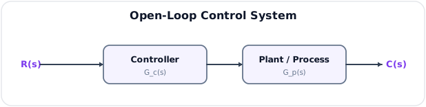
Mathematically, if controller transfer function is \(G_c(s)\) and plant transfer function is \(G_p(s)\):
Examples
| System | Why Open Loop? |
|---|---|
| Electric toaster | Heating time is preset; toast color is not measured |
| Washing machine timer | Wash cycle runs for fixed time regardless of cleanliness |
| Traffic signal timer | Signal changes based on preset timing, not actual traffic density |
| Open-loop stepper motor | Input pulses command position, but actual position is not measured |
Advantages
- Simple construction
- Low cost
- Easy maintenance
- Generally stable because there is no feedback loop
- No sensor required
- Faster response when calibration is accurate
Disadvantages
- Cannot correct errors automatically
- Sensitive to disturbances
- Sensitive to parameter variations
- Less accurate than closed-loop systems
- Requires recalibration
- Cannot compensate for load changes
3. Closed-Loop Control System
Likely Exam Question (10 marks)
"Explain closed-loop control system with block diagram. Derive the closed-loop transfer function for negative feedback."
A closed-loop control system is a control system in which the control action depends on the output.
The output is measured, compared with the reference input, and the error is used to generate corrective action.
Basic negative-feedback block diagram:
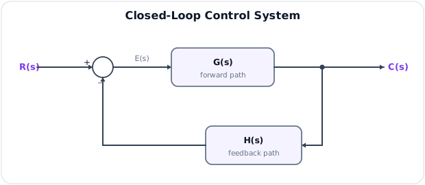
where:
- \(G(s)\) = forward-path transfer function
- \(H(s)\) = feedback-path transfer function
- \(R(s)\) = reference input
- \(C(s)\) = output
- \(E(s)\) = error signal
Derivation of Closed-Loop Transfer Function
For negative feedback:
Substitute:
Therefore:
This is the standard transfer function of a negative-feedback closed-loop system.
For unity feedback, \(H(s)=1\):
For positive feedback:
Advantages
- Higher accuracy
- Automatic error correction
- Reduced effect of disturbances
- Reduced sensitivity to parameter variations
- Increased bandwidth
- Better linearity
Disadvantages
- More complex than open-loop systems
- Higher cost due to sensors and feedback components
- May become unstable if badly designed
- Requires careful analysis of stability and compensation
- Feedback may introduce noise if sensor signal is noisy
4. Open-Loop vs Closed-Loop Systems
Likely Exam Question (5 marks)
"Compare open-loop and closed-loop control systems."
| Feature | Open-Loop System | Closed-Loop System |
|---|---|---|
| Feedback | Not present | Present |
| Control action | Independent of output | Depends on output |
| Error correction | Not automatic | Automatic |
| Accuracy | Lower | Higher |
| Sensitivity to disturbance | High | Low |
| Sensitivity to parameter variation | High | Low |
| Stability | Usually stable | May become unstable |
| Complexity | Simple | More complex |
| Cost | Low | Higher |
| Calibration | Required often | Less frequent |
| Example | Toaster, timer-based washer | Thermostat, speed control, autopilot |
Key Idea
Open-loop systems are useful when the relationship between input and output is accurately known and disturbances are negligible.
Closed-loop systems are preferred when accuracy, disturbance rejection, and robustness are important.
5. Feedback in Control Systems
Likely Exam Question (5 marks)
"What is feedback? Explain the effects of negative feedback in control systems."
Feedback is the process of taking a portion of the output and feeding it back to the input for comparison with the reference.
Types of Feedback
| Type | Error Signal | Effect |
|---|---|---|
| Negative feedback | \(E(s)=R(s)-H(s)C(s)\) | Reduces error and improves stability |
| Positive feedback | \(E(s)=R(s)+H(s)C(s)\) | Increases effective gain; may cause instability |
Effects of Negative Feedback
Negative feedback generally:
- Improves accuracy
- Reduces steady-state error
- Reduces sensitivity to parameter variations
- Reduces effect of disturbances
- Increases bandwidth
- Improves linearity
- May reduce overall gain
- May cause instability if phase shift becomes excessive
Loop Gain
The product \(G(s)H(s)\) is called loop gain.
Loop gain determines sensitivity, stability margins, and accuracy.
For large loop gain:
Thus the closed-loop behavior depends mainly on the feedback element, not plant variation.
6. Classification of Control Systems
Likely Exam Question (5 marks)
"Classify control systems with suitable examples."
Linear and Nonlinear Systems
A linear system satisfies superposition:
Examples: ideal RLC circuits, small-signal amplifier models, linearized motor control systems.
A nonlinear system does not satisfy superposition.
Examples: saturation, dead zone, backlash, relay control, diode circuits, magnetic hysteresis.
Time-Invariant and Time-Varying Systems
A time-invariant system has parameters that do not change with time.
Example: fixed RLC network.
A time-varying system has parameters that change with time.
Example: missile mass changes as fuel burns.
Continuous-Time and Discrete-Time Systems
| Type | Signal Nature | Example |
|---|---|---|
| Continuous-time | Signals defined for all time | Analog motor speed control |
| Discrete-time | Signals sampled at intervals | Digital control using microcontroller |
SISO and MIMO Systems
| Type | Meaning | Example |
|---|---|---|
| SISO | Single input, single output | Heater temperature control |
| MIMO | Multiple input, multiple output | Aircraft control system |
Regulator and Tracking System
A regulator keeps output constant despite disturbances.
Example: voltage regulator.
A tracking system makes output follow a changing input.
Example: radar antenna tracking a target.
7. Servomechanism
Likely Exam Question (5 marks)
"What is a servomechanism? Explain its components and applications."
A servomechanism is a closed-loop control system in which the output is mechanical position, velocity, or acceleration.
It uses feedback to make the mechanical output follow the input command accurately.
Basic Servo System
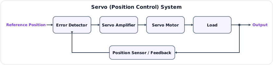
Components
| Component | Function |
|---|---|
| Error detector | Compares desired and actual position |
| Servo amplifier | Amplifies error signal |
| Servo motor | Converts electrical signal into mechanical motion |
| Load | Mechanical system to be positioned |
| Feedback sensor | Measures position or speed |
Examples
- Radar antenna positioning
- CNC machine tool positioning
- Robotic arm control
- Aircraft control surfaces
- Disk-drive head positioning
- Automatic steering systems
DC and AC Servomotors
| Feature | DC Servomotor | AC Servomotor |
|---|---|---|
| Supply | DC | AC |
| Control | Armature or field control | Usually control-phase voltage |
| Response | Fast and easy to control | Smooth, reliable, less maintenance |
| Maintenance | Brushes require maintenance | No brushes in many types |
| Applications | Robotics, position control | Instrument servos, low-power control |
8. System Stability
Likely Exam Question (10 marks)
"Define stability of a control system. Explain absolute stability, relative stability, and BIBO stability."
Stability is the most important requirement of a control system.
A system is stable if its output remains bounded for a bounded input and if natural response dies out with time.
BIBO Stability
A system is BIBO stable if every bounded input produces a bounded output.
Stability from Pole Locations
For a continuous-time linear time-invariant system, stability depends on closed-loop pole locations.
| Pole Location | System Behavior |
|---|---|
| All poles in left half of \(s\)-plane | Stable |
| Any pole in right half of \(s\)-plane | Unstable |
| Simple pole on imaginary axis, none in right half-plane | Marginally stable |
| Repeated pole on imaginary axis | Unstable |
Absolute and Relative Stability
Absolute stability answers whether the system is stable or unstable.
Relative stability measures how stable the system is, such as:
- Distance of dominant poles from imaginary axis
- Damping ratio \(\zeta\)
- Settling time
- Gain margin
- Phase margin
Characteristic Equation
For a closed-loop system:
The characteristic equation is:
Closed-loop poles are roots of this equation.
9. Sensitivity
Likely Exam Question (10 marks)
"Define sensitivity. Show that negative feedback reduces sensitivity of closed-loop transfer function to forward-path gain variation."
Sensitivity measures how much a system transfer function changes due to change in a parameter.
Sensitivity of \(T\) with respect to parameter \(K\) is:
Sensitivity of Closed-Loop System to Forward Gain
For negative feedback:
Sensitivity of \(T\) with respect to \(G\):
Differentiate:
Also:
Therefore:
For open-loop system, \(T=G\), so:
Thus negative feedback reduces sensitivity by the factor:
Sensitivity to Feedback Element
For \(T = G/(1+GH)\):
If \(GH \gg 1\):
This means the closed-loop transfer function becomes highly dependent on the feedback element. Therefore, feedback elements must be accurate and stable.
10. Disturbance Rejection
Likely Exam Question (5 marks)
"Explain how feedback reduces the effect of disturbance in a control system."
Consider a disturbance \(D(s)\) entering at the plant output of a unity-feedback system:
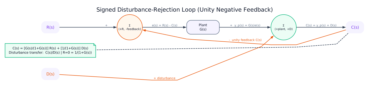
The output due to input and disturbance is:
The disturbance effect is reduced by:
Thus high loop gain improves disturbance rejection.
11. Control-System Components
Error Detector
An error detector compares reference and feedback signals. Examples:
- Potentiometer pair in position control
- Synchro pair in AC position control
- Differential amplifier in electronic control
Controller
The controller processes the error signal and produces control input for the plant.
Common controllers:
| Controller | Transfer Function | Main Effect |
|---|---|---|
| Proportional (P) | \(K_p\) | Improves speed but may leave steady-state error |
| Integral (I) | \(K_i/s\) | Eliminates steady-state error but may reduce stability |
| Derivative (D) | \(K_ds\) | Predictive action; improves damping |
| PI | \(K_p + K_i/s\) | Eliminates steady-state error |
| PD | \(K_p + K_ds\) | Improves transient response |
| PID | \(K_p + K_i/s + K_ds\) | Combines accuracy and damping |
Actuator
An actuator converts controller output into physical action.
Examples:
- DC motor
- Hydraulic actuator
- Pneumatic actuator
- Solenoid valve
- Power amplifier
Sensor
A sensor measures the output or state of the system.
Examples:
- Tachogenerator for speed
- Potentiometer or encoder for position
- Thermocouple or RTD for temperature
- Pressure transducer for pressure
12. Solved Examples
Example 1 - Closed-Loop Transfer Function
Q. A system has forward-path transfer function \(G(s)=\frac{100}{s+10}\) and feedback transfer function \(H(s)=0.1\). Find the closed-loop transfer function.
Solution:
Example 2 - Sensitivity Reduction
Q. A closed-loop system has loop gain \(GH=99\). Find sensitivity of closed-loop transfer function to forward gain variation.
Solution:
Thus a 10% change in \(G\) causes only 0.1% change in closed-loop transfer function.
Example 3 - Stability from Poles
Q. Determine stability for systems with the following pole sets:
- \(s=-2,-5\)
- \(s=-1, +3\)
- \(s=\pm j4\)
- \(s=0,0,-2\)
Solution:
| Poles | Stability | Reason |
|---|---|---|
| \(-2,-5\) | Stable | All poles in left half-plane |
| \(-1,+3\) | Unstable | One pole in right half-plane |
| \(\pm j4\) | Marginally stable | Simple imaginary-axis poles |
| \(0,0,-2\) | Unstable | Repeated pole on imaginary axis |
13. Quick Revision Table
| Topic | Key Result |
|---|---|
| Open-loop system | Control action independent of output |
| Closed-loop system | Control action depends on output via feedback |
| Negative-feedback transfer function | \(T(s)=G(s)/(1+G(s)H(s))\) |
| Positive-feedback transfer function | \(T(s)=G(s)/(1-G(s)H(s))\) |
| Loop gain | \(L(s)=G(s)H(s)\) |
| Characteristic equation | \(1+G(s)H(s)=0\) |
| BIBO stability | Bounded input gives bounded output |
| Stable pole condition | All closed-loop poles in left half-plane |
| Sensitivity to forward gain | \(S_G^T=1/(1+GH)\) |
| Sensitivity to feedback element | \(S_H^T=-GH/(1+GH)\) |
| Disturbance reduction | Disturbance effect reduced by \(1/(1+G)\) |
Key Exam Points - Fundamentals
- Open-loop systems are simple but inaccurate under disturbances.
- Closed-loop systems use feedback to reduce error and sensitivity.
- Negative feedback reduces forward-path sensitivity by \(1+GH\).
- The characteristic equation \(1+G(s)H(s)=0\) decides closed-loop stability.
- A stable continuous-time system must have all closed-loop poles in the left half-plane.
Model Answer — Control-System Definition and Classification [5 marks]
Exam-ready answer
A control system is an interconnection of components arranged to make a plant output \(c(t)\) follow a desired reference \(r(t)\) despite parameter changes and disturbances. The plant is the physical process; a controller computes the action, an actuator supplies power, and a sensor measures the controlled variable. For negative feedback, define the summing-junction sign convention
where \(e\) is tracking error and \(*\) denotes convolution. Signal units depend on the application: for position control, \(r,c\) may be radians and actuator output may be N·m; transfer functions themselves carry the output/input unit ratio.
Control systems are classified as follows:
| Basis | Classes and defining feature |
|---|---|
| Feedback | Open loop: action is independent of measured output. Closed loop: output is sensed and compared with reference. |
| Linearity | Linear: superposition holds. Nonlinear: saturation, backlash, dead zone or nonlinear equations violate it. |
| Time dependence | Time invariant: parameters do not change with time. Time varying: one or more parameters explicitly vary. |
| Signal time | Continuous time: signals exist at every instant. Discrete/digital: signals are sampled and controller usually computes at sample instants. |
| Uncertainty | Deterministic: inputs/parameters are prescribed. Stochastic: random variables or noise are modeled statistically. |
| Number of channels | SISO: one input and one output. MIMO: multiple interacting inputs or outputs. |
| Parameter distribution | Lumped: state varies only with time. Distributed: state also varies spatially, leading to partial differential equations. |
For an LTI SISO closed loop with forward path \(G(s)\) and feedback \(H(s)\),
This derivation states the zero-initial-condition assumption used by transfer functions and fixes the negative-feedback sign.
Check/application: a timer-operated toaster is open loop because it does not measure browning; a thermostat-controlled heater is closed loop because temperature is measured and compared with the setting. A practical plant can belong to several classes simultaneously, for example a continuous-time, nonlinear, time-invariant MIMO aircraft. Classification guides the analysis method but is not itself a performance guarantee: a closed loop can still be inaccurate or unstable if badly designed.
Practice target: 8–9 minutes; define the signal roles, state the negative summing sign, and classify by at least five independent bases.
Model Answer — Open-Loop and Closed-Loop Systems [5 marks]
Exam-ready answer
An open-loop system applies a command without measuring the actual output; its control action is independent of output and cannot automatically correct error.
If controller and plant combine to \(G(s)\) under zero initial conditions,
A closed-loop system measures the output and feeds \(B(s)=H(s)C(s)\) back for comparison. With negative feedback, define \(E=R-B\) and \(C=GE\). Then
| Feature | Open loop | Closed loop with negative feedback |
|---|---|---|
| Output measurement | Absent | Present through sensor \(H\) |
| Accuracy/disturbance correction | Depends on calibration; cannot self-correct | Error drives correction; rejects many disturbances |
| Parameter sensitivity | Directly sensitive to plant change | Usually reduced by loop factor \(1+GH\) |
| Complexity and cost | Low | Higher: sensor, comparator and controller |
| Bandwidth | Usually smaller for comparable plant | Often increased when stable |
| Stability | No feedback-induced instability | Can become unstable if loop phase/gain is poor |
| Examples | Timed washer, traffic-light timer, toaster timer | Motor-speed control, voltage regulator, thermostat |
Worked check: let \(G=100\) and unity feedback \(H=1\) at low frequency. Open-loop output gain is 100 and a 10% plant change produces about a 10% output-gain change. Closed-loop gain is \(100/101=0.990\), close to the desired unity value, and its normalized sensitivity to \(G\) is \(1/(1+100)=0.0099\); a 10% plant change causes only about 0.099% closed-loop-gain change.
Closed loop is preferred when accuracy and disturbance rejection justify extra hardware, but sensor noise, actuator limits and delay remain. Open loop is suitable when the input-output relation is predictable and output measurement is unnecessary or uneconomical. Feedback does not automatically ensure stability; the characteristic equation \(1+G(s)H(s)=0\) must be checked.
Practice target: 9 minutes; draw both diagrams, derive the closed-loop denominator, and compare at least six features with examples.
Model Answer — Effects of Feedback on System Performance [10 marks]
Exam-ready answer
Assume a linear time-invariant SISO system with negative feedback. Define \(E=R-HC\), \(C=GE\) and loop transfer \(L=GH\). Solving gives
and the closed-loop poles are roots of \(1+L(s)=0\). The plus sign in the denominator follows from the negative sign at the summing junction; positive feedback would give \(1-GH\).
Gain and accuracy. Negative feedback reduces nominal gain from \(G\) to \(G/(1+L)\). When \(|L|\gg1\) and the loop is stable, \(T\approx1/H\), so tracking depends mainly on the feedback element and steady error is reduced. The price is that more forward gain is required.
Sensitivity. The normalized sensitivity of \(T\) to \(G\) is
The sensitivity to \(H\) is
Thus large loop gain suppresses forward-path parameter variation but makes the result depend on sensor calibration.
Disturbance rejection. For unity feedback with a disturbance \(D\) added positively at the plant output, let \(C=G(R-C)+D\). Therefore
The disturbance sign and transfer change if it enters at a different point; one must not quote \(1/(1+G)\) without locating it. Measurement noise injected in the feedback path can pass approximately as \(-G/(1+GH)\), so high loop gain does not reject every unwanted signal.
Bandwidth and transient response. For the illustrative first-order plant \(G(s)=K/(1+s\tau)\) with constant feedback \(H\), the closed loop is
Hence the time constant becomes \(\tau_c=\tau/(1+KH)\) and bandwidth increases approximately by \(1+KH\), while low-frequency gain decreases by the same factor. Negative feedback also tends to reduce distortion generated inside the forward path by the loop factor.
Stability. Feedback moves poles; it is stabilizing only with adequate gain and phase margins. Transport delay and high-frequency pole phase lag can turn the returning signal effectively positive, causing oscillation. Therefore the characteristic equation, Routh/root-locus test, or Bode/Nyquist margins must be examined.
Check: if \(L=99\) at low frequency, \(S_G^T=0.01\); a 10% change in \(G\) produces about a 0.1% change in \(T\). This benefit is meaningful only where the loop remains stable and unsaturated. Negative feedback is used in regulators, servos and amplifiers, but actuator saturation, sensor noise and unmodeled dynamics limit achievable gain and bandwidth.
Practice target: 18 minutes; derive gain and both sensitivities, label the disturbance insertion point, and state the bandwidth-versus-stability tradeoff.
Model Answer — System Stability and Sensitivity [5 marks]
Exam-ready answer
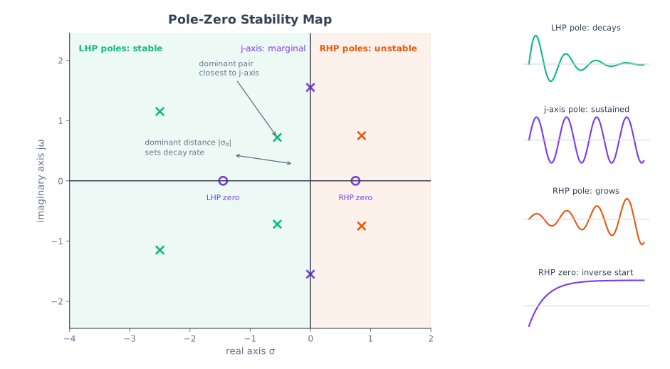
A continuous-time system is BIBO stable if every bounded input produces a bounded output. For a proper rational LTI transfer function with no hidden unstable pole-zero cancellation, BIBO stability requires every closed-loop pole to lie strictly in the open left half of the \(s\)-plane:
Poles in the right half-plane give growing exponentials and instability. A repeated pole on the imaginary axis is unstable. Simple imaginary-axis poles may give a bounded zero-input oscillation and are called marginally stable in internal-response terminology, but they do not satisfy strict BIBO stability because a resonant bounded input can produce unbounded output. Absolute stability asks stable or unstable; relative stability asks how far poles and frequency margins are from the boundary.
For negative feedback, with \(E=R-HC\) and \(C=GE\),
is the characteristic equation that determines stability.
Sensitivity measures fractional output-model change caused by a fractional parameter change. Its normalized definition is
For \(x=G\),
Therefore negative feedback with large, well-phased loop gain reduces sensitivity to forward-path variation. It does not remove sensitivity to all quantities: \(S_H^T=-GH/(1+GH)\) approaches \(-1\) at high gain.
Check: poles \(-2\) and \(-5\) give a stable response; poles \(-2\) and \(+1\) are unstable; a repeated pole at the origin is unstable. If \(GH=49\), then \(S_G^T=1/50=0.02\), so a 5% gain change causes approximately a 0.1% closed-loop change. Pole tests assume the model includes all relevant dynamics; delays, nonlinear saturation and hidden internal modes can invalidate a transfer-function-only conclusion.
Practice target: 9 minutes; distinguish BIBO from marginal stability, state the pole condition, and derive normalized sensitivity rather than only quoting it.