Signals and Their Classification
Possible Exam Questions
Exam Questions and Answer Map
Evidence note: [PYQ paper/year] = exact question observed in that past paper; [likely] = pattern-predicted variant not confirmed as exact PYQ.
-
Classify signals (deterministic/random, energy/power, periodic/aperiodic, even/odd). [5] — [likely]
-
Answer plan: Define continuous vs discrete time → define periodic (\(x(t)=x(t+T)\)) vs aperiodic → define energy (\(E<\infty\)) vs power (\(P<\infty\)) signal → define even/odd and deterministic/random → give one example of each.
-
Model answer: Classification of Signals
-
Differentiate between energy and power signals with examples. [5] — [likely]
-
Answer plan: Write energy and power definitions → state \(0<E<\infty\) (energy) vs \(0<P<\infty\) (power) → note a signal cannot be both → give finite pulse (energy) and sinusoid (power) examples with worked \(E\) and \(P\).
-
Model answer: Energy and Power Signals
-
Define the unit step, delta, sinc and signum functions and give their transforms. [5] — [likely]
-
Answer plan: Define each function mathematically → state \(\delta(t)\to 1\), \(u(t)\to\pi\delta(\omega)+1/j\omega\), \(\text{sinc}(t)\to\text{rect}(\omega/2\pi)\), \(\text{sgn}(t)\to 2/j\omega\) → sketch each waveform.
-
Model answer: Unit Step, Delta, Sinc and Signum
-
Define the Dirac delta (unit impulse) function and explain its important mathematical properties. [5–10] — [likely]
-
Answer plan: Define \(\delta(t)\) by unit area and \(\delta(t)=0\) for \(t\neq0\) → state sifting → state scaling \(\delta(at)=\delta(t)/\lvert a\rvert\) → state \(\delta(t)=du/dt\) → state convolution identity \(x*\delta=x\) → give the discrete equivalent.
- Model answer: Dirac Delta and Its Properties
1. Signal Classification
Likely Exam Question (5 marks)
"Classify signals with examples: continuous/discrete, periodic/aperiodic, energy/power, even/odd, deterministic/random."
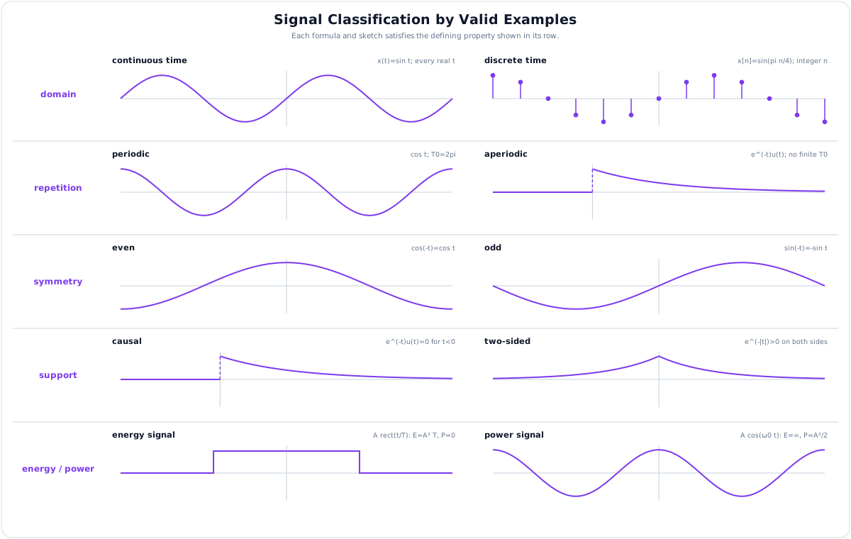
A signal is a function that carries information about the behaviour of a physical system. Before analysing signals with convolution or transforms, they are grouped by a few standard properties.
Continuous-Time and Discrete-Time Signals
- A continuous-time (CT) signal \(x(t)\) is defined for every value of time \(t\) on a continuous axis.
- A discrete-time (DT) signal \(x[n]\) is defined only at integer indices \(n\); it is usually obtained by sampling a CT signal.
If, in addition, the amplitude takes only a finite set of values, the signal is digital; if the amplitude is continuous, it is analog.
Periodic and Aperiodic Signals
A signal is periodic if it repeats after a fixed interval:
The smallest such \(T_0\) (or integer \(N\)) is the fundamental period. A signal that satisfies no such relation is aperiodic. A DT sinusoid \(\cos(\Omega n)\) is periodic only when \(\Omega/2\pi\) is rational.
Even and Odd Signals
An even signal is symmetric about the vertical axis (e.g. \(\cos t\), \(\lvert t\rvert\)); an odd signal is anti-symmetric about the origin (e.g. \(\sin t\), \(t\)). Any signal can be split into an even and an odd part:
Deterministic and Random Signals
- A deterministic signal can be described by an exact mathematical expression, so its value is known at every instant (e.g. a carrier \(A\cos\omega_c t\)).
- A random (stochastic) signal cannot be predicted exactly and is described only by statistics such as mean and autocorrelation (e.g. noise, a real message waveform).
Causal, Anti-causal and Two-sided Signals
- Causal: \(x(t)=0\) for \(t<0\) (starts at or after the origin).
- Anti-causal: \(x(t)=0\) for \(t>0\).
- Two-sided: non-zero for both \(t<0\) and \(t>0\).
2. Energy and Power Signals
Likely Exam Question (5 marks)
"Differentiate between energy and power signals with examples."
Continuous-Time Energy and Power
Signal energy:
Average power:
Discrete-Time Energy and Power
Signal energy:
Average power:
Comparison
An energy signal satisfies \(0<E<\infty\) and consequently has zero average power. A power signal satisfies \(0<P<\infty\) and normally has infinite total energy.
| Signal Type | Energy | Average Power | Example |
|---|---|---|---|
| Energy signal | \(0<E<\infty\) | \(0\) | finite-duration pulse |
| Power signal | \(\infty\) | \(0<P<\infty\) | sinusoid, periodic square wave |
A signal cannot be both an energy signal and a power signal, except the zero signal.
Energy-signal example. Let \(x(t)=A\) for \(\lvert t\rvert\leq T/2\) and zero elsewhere. Then
Power-signal example. For \(x(t)=A\cos\omega_0t\), average the squared signal over one period \(T_0\):
Thus finite-duration signals are usually energy signals, while non-decaying periodic signals are power signals.
3. Elementary Signals
Likely Exam Question (5 marks)
"Define unit step, ramp, signum, and sinc functions. State their transforms and uses."
A handful of standard (elementary) signals are the building blocks used throughout signal and system analysis. The unit impulse is treated separately in Section 4.
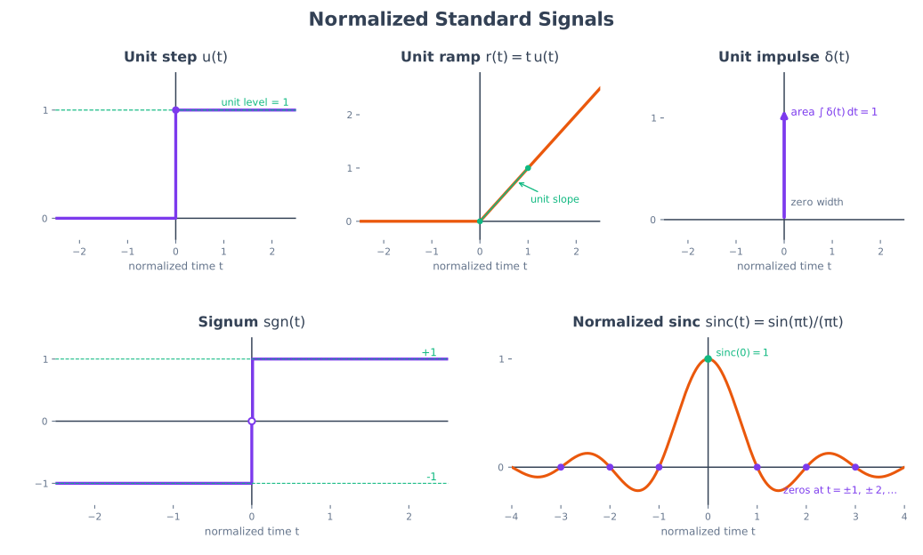
Unit Step Function
The unit step models switching action and causal signal starting points.
Its Fourier transform is understood in the distribution sense:
It is used to switch signals on at a specified time; for example, \(x(t)u(t-t_0)\) represents a signal beginning at \(t=t_0\).
Unit Ramp Function
The ramp, step and impulse form an integral–derivative chain:
so \(\delta(t)=d^2r(t)/dt^2\). The ramp models a linearly rising input such as a constant-rate sweep.
Signum Function
Relationship:
Using \(\operatorname{sgn}(t)=2u(t)-1\) and the transforms of \(u(t)\) and \(1\),
The signum function describes bipolar switching and is useful when representing symmetric discontinuities and deriving Hilbert-transform relations.
Here \(\operatorname{PV}\) denotes the Cauchy principal-value distribution; it is required because \(1/\omega\) is singular at \(\omega=0\).
Sinc Function
Normalized sinc function:
Sinc functions appear in sampling theory, ideal low-pass filters, and rectangular pulse spectra.
With the normalized definition above and the angular-frequency Fourier-transform convention,
This pair explains why an ideal rectangular low-pass spectrum produces a sinc-shaped impulse response and why ideal band-limited interpolation uses shifted sinc functions.
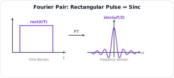
Classic Fourier pair — a rectangular pulse in time ↔ a sinc in frequency (a narrow pulse ⇒ a wide spectrum).
Exponential Signals
The real exponential \(x(t)=Ce^{at}\) grows when \(a>0\) and decays when \(a<0\); the decaying form \(e^{-at}u(t)\) is the most common building block of causal responses.
The complex exponential is the eigenfunction of every LTI system and, by Euler's identity, contains the sinusoids:
The discrete-time counterpart is \(x[n]=Cr^{n}\) (real) or \(e^{j\Omega n}\) (complex). Because an LTI system merely scales a complex exponential by \(H(\omega)\) or \(H(z)\), these signals are the natural basis for the Fourier, Laplace and Z transforms in later chapters.
4. The Unit Impulse Function
Likely Exam Question (5–10 marks)
"Define the Dirac delta (unit impulse) function and explain its important mathematical properties."
Continuous-Time Impulse \(\delta(t)\)
The Dirac delta, or continuous-time unit impulse, is not an ordinary function with a finite value at every instant. It is a generalized function (distribution) defined by how it behaves inside an integral. It is zero for every \(t\neq 0\), is concentrated at \(t=0\), and has total area equal to one:
It may be visualized as the limiting form of a rectangular pulse whose width approaches zero while its height increases so that its area remains one:
Thus, saying that \(\delta(0)\) is "infinite" is only a useful sketching idea; its rigorous meaning comes from the following integral properties.
1. Unit-Area and Shifting Property
The unshifted impulse is located at the origin and has unit area. Replacing \(t\) by \(t-t_0\) shifts it to \(t=t_0\) without changing its area:
More generally, an impulse has area one over any integration interval containing \(t_0\), and area zero over an interval that does not contain \(t_0\). A weighted impulse \(A\delta(t-t_0)\) therefore represents an impulse at \(t_0\) having area (or strength) \(A\).
2. Sifting or Sampling Property
If \(x(t)\) is continuous at \(t=t_0\), multiplication by \(\delta(t-t_0)\) and integration over an interval containing \(t_0\) extracts only the value of \(x(t)\) at that instant:
This happens because the impulse is zero everywhere except at \(t_0\). Hence all values of \(x(t)\) away from \(t_0\) make no contribution, while the unit area of the impulse leaves precisely \(x(t_0)\). With a weighted impulse,
This is called sifting because the impulse "sifts out" one value from the complete signal.
3. Multiplication or Sampling Identity
Before integration, the same idea is written as the distribution identity
The factor \(x(t)\) can be replaced by the constant \(x(t_0)\) because the product survives only at the location of the impulse. This identity is valid when interpreted under an integral; the two sides produce the same result against every test function.
4. Time-Scaling Property
For any non-zero real constant \(a\),
To see why the reciprocal factor is necessary, let \(u=at\). Changing variables in the impulse integral must preserve unit area:
The absolute value is essential because reversing the time axis must not produce a negative impulse area. The useful shifted form is
Therefore, compression of the time argument increases the apparent width compression but reduces the impulse weight by \(1/\lvert a\rvert\) so that the distribution transforms consistently.
5. Even Symmetry
Setting \(a=-1\) in the scaling property gives
Thus the impulse is an even signal. Time reversal leaves both its location at the origin and its unit area unchanged.
6. Relation to the Unit-Step Function
The unit impulse is the generalized derivative of the unit step \(u(t)\):
Conversely, accumulating impulses from \(-\infty\) to \(t\) produces the unit step:
The step changes instantaneously by one unit at the origin, so its derivative is concentrated there and has area equal to the size of the jump. More generally, a jump of magnitude \(A\) at \(t=t_0\) contributes \(A\delta(t-t_0)\) to the derivative.
7. Derivative of an Impulse
The derivative \(\delta'(t-t_0)\) samples the negative derivative of a differentiable function:
Using integration by parts,
because the boundary term is zero and the remaining integral follows directly from the sifting property.
8. Identity Under Convolution
The unit impulse acts as the identity element of convolution:
A shifted impulse shifts the signal by the same amount:
This property is fundamental in LTI-system analysis: an arbitrary signal can be regarded as a continuous collection of shifted impulses, and the corresponding output is a collection of shifted impulse responses.
9. Fourier- and Laplace-Transform Property
Using the sifting property,
Similarly,
Therefore, an ideal impulse has a flat spectrum: it contains all frequency components with equal magnitude and is useful for testing the frequency response of a system.
Solved Example - Combined Scaling and Sifting
Q. Evaluate
Solution. First express the impulse in standard shifted form:
Now apply the sifting property:
Common Exam Mistakes
- Do not omit the absolute value in \(\delta(at)=\delta(t)/\lvert a\rvert\).
- \(\delta(t-t_0)\) is located at \(t=+t_0\), not at \(-t_0\).
- The continuous-time impulse is not an ordinary pulse with a finite height; its area and action under integration define it.
- Apply sifting only when the impulse location lies inside the limits of integration.
Since \(\int\delta(t)\,dt = 1\) is dimensionless, \(\delta(t)\) has units of \(1/\text{time}\).
Discrete-Time Impulse \(\delta[n]\)
Unlike the continuous case, the discrete unit impulse (unit sample) is an ordinary, well-defined sequence:
A shift \(\delta[n-n_0]\) moves the only non-zero sample from \(n=0\) to \(n=n_0\). Therefore,
and the discrete sifting property is
Only the term at \(n=n_0\) survives in the sum. Equivalently,
The sequence is even because \(\delta[-n]=\delta[n]\). Its relation to the discrete unit step is a first difference, rather than a derivative:
Finally, it is the identity element for discrete convolution:
Every discrete-time sequence can consequently be decomposed into scaled, shifted unit samples:
This decomposition is the direct bridge from the unit impulse to convolution and the impulse-response description of an LTI system (next chapters).
Key Exam Points - Signals & Classification
- Energy signal: \(0<E<\infty\), \(P=0\) (finite pulse). Power signal: \(0<P<\infty\), \(E=\infty\) (sinusoid).
- Any signal splits into even + odd parts: \(x_e=\tfrac12[x(t)+x(-t)]\), \(x_o=\tfrac12[x(t)-x(-t)]\).
- Ramp–step–impulse chain: \(\delta(t)=du/dt\), \(u(t)=dr/dt\).
- Sifting: \(\int x(t)\delta(t-t_0)\,dt=x(t_0)\); scaling: \(\delta(at)=\delta(t)/\lvert a\rvert\).
- Convolution identity: \(x(t)*\delta(t)=x(t)\); \(\mathcal{F}\{\delta(t)\}=1\) (flat spectrum).
Model Answer — Classification of Signals [5 marks]
Exam-ready answer
A signal is a function that conveys information about a physical phenomenon; \(x(t)\) denotes a continuous-time (CT) signal and \(x[n]\) a discrete-time (DT) sequence. Signals are classified by independent tests, so one signal can belong to several classes at once.
| Classification | Defining test | Example |
|---|---|---|
| Deterministic / random | Exactly specified by a rule / described statistically | \(A\cos\omega_0t\) / thermal noise |
| Periodic / aperiodic | \(x(t+T_0)=x(t)\) for some least \(T_0>0\) / no such \(T_0\) | cosine / decaying exponential |
| Energy / power | \(0<E<\infty\) / \(0<P<\infty\) | finite pulse / periodic sinusoid |
| Even / odd | \(x(-t)=x(t)\) / \(x(-t)=-x(t)\) | \(\cos t\) / \(\sin t\) |
| Causal / noncausal | \(x(t)=0\) for \(t<0\) / nonzero before the origin | \(e^{-t}u(t)\) / \(e^{-\lvert t\rvert}\) |
The CT energy and average power tests are
with sums replacing integrals in DT. Every real or complex signal has a unique even–odd decomposition:
Indeed, substituting \(-t\) proves \(x_e(-t)=x_e(t)\) and \(x_o(-t)=-x_o(t)\). For example, if \(x(t)=1+t\), then \(x(-t)=1-t\), hence \(x_e(t)=1\) and \(x_o(t)=t\). A DT sinusoid \(\cos(\Omega_0n)\) is periodic only if \(\Omega_0/(2\pi)\) is rational; this is an important difference from CT sinusoids.
Practice target: 8 minutes; write the five defining tests, the even–odd formulas and at least one example of every class.
Model Answer — Energy and Power Signals [5 marks]
Exam-ready answer
For a CT signal \(x(t)\), total energy and time-average power are
For a DT signal, use \(E=\sum_{n=-\infty}^{\infty}|x[n]|^2\) and \(P=\lim_{N\to\infty}(2N+1)^{-1}\sum_{n=-N}^{N}|x[n]|^2\). These definitions assume the indicated limit exists.
| Type | Energy | Average power | Typical signal |
|---|---|---|---|
| Energy signal | \(0<E<\infty\) | \(P=0\) | finite-duration pulse or decaying transient |
| Power signal | \(E=\infty\) | \(0<P<\infty\) | nonzero periodic signal |
| Neither | \(E=\infty\) and \(P\) is zero, infinite or undefined | not classified as either | \(x(t)=t\) |
Except for the zero signal, a signal cannot be both: finite \(E\) divided by an interval of unbounded length gives \(P=0\), whereas positive finite \(P\) accumulated for infinite time gives \(E=\infty\).
Energy example: let \(x(t)=A\) for \(|t|\le T_0/2\) and zero otherwise. Then
Power example: for \(x(t)=A\cos\omega_0t\), average over one period \(T_p=2\pi/\omega_0\):
while its energy diverges. Thus duration or decay decides energy behaviour, whereas sustained repetition normally decides power behaviour.
Practice target: 8 minutes; give both CT and DT definitions and calculate one finite-pulse energy and one sinusoidal power.
Model Answer — Unit Step, Delta, Sinc and Signum [5 marks]
Exam-ready answer
Using the angular-frequency convention \(X(\omega)=\int_{-\infty}^{\infty}x(t)e^{-j\omega t}dt\), the four standard signals and their Fourier transforms are:
| Signal | Definition | Fourier transform |
|---|---|---|
| Unit step | \(u(t)=0\) for \(t<0\), \(u(t)=1\) for \(t>0\) | \(\pi\delta(\omega)+\operatorname{PV}(1/j\omega)\) |
| Unit impulse | \(\delta(t)=0\) for \(t\ne0\), \(\int\delta(t)dt=1\) | \(1\) |
| Normalized sinc | \(\operatorname{sinc}(t)=\sin(\pi t)/(\pi t)\), with value \(1\) at \(t=0\) | \(\operatorname{rect}(\omega/2\pi)\) |
| Signum | \(\operatorname{sgn}(t)=-1,0,1\) as \(t<0,t=0,t>0\) | \(2\operatorname{PV}(1/j\omega)\) |
Here \(\operatorname{PV}\) is the Cauchy principal value, needed because \(1/\omega\) is singular. The relations
explain the transform pairs: differentiation gives \(j\omega U(\omega)=1\) away from the origin, while the DC term required by the step contributes \(\pi\delta(\omega)\); substituting \(2u-1\) cancels the delta terms and leaves \(2/(j\omega)\). Directly, the impulse transform follows by sifting:
so the unshifted impulse has a flat spectrum. The sinc–rectangle pair states that an ideal rectangular low-pass spectrum has a sinc impulse response; narrower time support means wider frequency support. Unit steps model switching, impulses test LTI systems, sinc functions reconstruct band-limited signals, and signum represents bipolar switching.
Practice target: 9 minutes; draw the four waveforms, state the transform convention and include the two relations used to obtain the pairs.
Model Answer — Dirac Delta and Its Properties [5–10 marks]
5-mark answer and 10-mark extension
For 5 marks — write this
The Dirac delta \(\delta(t)\) is a generalized function, not an ordinary finite-height pulse. It is defined by
Its rigorous meaning is its action under integration. For a function \(x(t)\) continuous at \(t_0\), the sifting property is
The essential properties are
Thus scaling changes impulse weight to preserve area, differentiation of a unit jump produces an impulse, and convolution with an impulse is the identity operation. In DT, \(\delta[n]=1\) at \(n=0\) and \(0\) otherwise, with \(\delta[n]=u[n]-u[n-1]\) and \(\sum_nx[n]\delta[n-n_0]=x[n_0]\).
Add for a 10-mark variant
Derive scaling by putting \(v=at-b\) in an integral. Since \(dt=dv/|a|\) after accounting for orientation,
which proves \(\delta(at-b)=|a|^{-1}\delta(t-b/a)\). The multiplication identity \(x(t)\delta(t-t_0)=x(t_0)\delta(t-t_0)\) follows because both sides give the same result against every test function.
For the derivative impulse, integration by parts gives
Any sequence can be decomposed into shifted samples,
which, by linearity and time invariance, leads directly to the LTI output \(y[n]=\sum_kx[k]h[n-k]\).
Worked example: evaluate
Since \(\delta(2t-4)=\tfrac12\delta(t-2)\),
The factor \(1/2\) and the positive impulse location \(t=2\) are both marks-bearing details. An impulse therefore provides an ideal broadband test input: its transform is unity, so the output spectrum of an LTI system is its transfer function itself.
Practice target: 9 minutes for the 5-mark core or 17 minutes for the full answer; always show unit area, sifting, absolute-value scaling and one evaluated integral.