Discrete Signal Processing
Possible Exam Questions
Exam Questions and Answer Map
Evidence note: [PYQ paper/year] = exact question observed in that past paper; [likely] = pattern-predicted variant not confirmed as exact PYQ.
-
Define the DFT and IDFT; compute the DFT of a short sequence (e.g. N = 4). [5–10] — [likely]
-
Answer plan: Write DFT formula \(X[k]=\sum_{n=0}^{N-1}x[n]W_N^{kn}\) → write IDFT → define twiddle factor \(W_N=e^{-j2\pi/N}\) → for N=4 compute \(W_4=e^{-j\pi/2}=-j\) → evaluate each \(X[k]\) by substitution → present result.
-
Model answer: DFT, IDFT and Four-Point Example
-
Explain the FFT; how does it reduce computation compared with the DFT? [5] — [likely]
-
Answer plan: State DFT requires \(N^2\) complex multiplications → FFT uses divide-and-conquer (radix-2 decimation-in-time) → splits N-point into two N/2-point DFTs → reduces to \(\frac{N}{2}\log_2 N\) multiplications → draw butterfly diagram → give numerical example (N=1024: 5 million → 5120).
-
Model answer: FFT Computation and Radix-2 DIT Flow
-
Explain circular convolution and its relation to linear convolution. [5] — [likely]
-
Answer plan: Define circular convolution \(x[n]\circledast h[n]=\sum_{m=0}^{N-1}x[m]h[(n-m)_N]\) → state DFT convolution property: \(\text{IDFT}\{X[k]\cdot H[k]\}\) gives circular not linear → explain zero-padding to length \(L+M-1\) makes circular = linear → state overlap-add/save methods.
-
Model answer: Circular and Linear Convolution
-
State Parseval's theorem; define signal energy and power. [5] — [likely]
-
Answer plan: State Parseval's: \(\sum|x[n]|^2=\frac{1}{N}\sum|X[k]|^2\) → define energy signal (\(E<\infty\), \(P=0\)) → define power signal (\(P<\infty\), \(E=\infty\)) → give continuous-time equivalents → classify examples (pulse = energy, periodic = power).
-
Model answer: Parseval's Theorem, Signal Energy and Power
-
Define auto-correlation and state its properties. [5] — [likely]
-
Answer plan: Define \(R_{xx}[l]=\sum x[n]x[n+l]\) → state properties: symmetric \(R_{xx}[-l]=R_{xx}[l]\), maximum at origin \(|R_{xx}[l]|\leq R_{xx}[0]\), \(R_{xx}[0]=\) signal energy/power → relate to PSD via Wiener-Khinchin theorem → state applications (radar, synchronization).
- Model answer: Autocorrelation and Its Properties
1. Discrete Fourier Transform (DFT)
Likely Exam Question (10 marks)
"Define DFT and IDFT. State important properties and explain their use in spectrum analysis."
DFT Definition
The Discrete Fourier Transform (DFT) converts a finite-length discrete-time sequence into a finite set of equally spaced frequency samples.
For an \(N\)-point sequence \(x[n]\):
The DFT assumes the time sequence is periodic with period \(N\).
Frequency Index Meaning
The spacing between adjacent DFT bins is
where \(F_s\) is the sampling frequency. Because discrete-time frequency is periodic with period \(F_s\), bins in the upper half of the DFT represent negative frequencies. In signed-frequency order,
For even \(N\), bin \(k=N/2\) is the Nyquist-frequency bin at \(F_s/2\), equivalently \(-F_s/2\). Thus \(k=0\) is DC, the lower bins are positive frequencies, and the upper bins wrap around to negative frequencies.
Matrix View
DFT uses the twiddle factor:
So:
In matrix form,
The DFT matrix contains sampled complex sinusoids. Each row correlates the input sequence with one frequency bin.
2. Inverse DFT (IDFT)
IDFT Definition
The IDFT reconstructs the time-domain samples from DFT coefficients:
DFT and IDFT form a transform pair:
Important DFT Properties
Let \((q)_N\) denote \(q\) reduced modulo \(N\). For \(x[n]\leftrightarrow X[k]\):
1. Linearity
The spectrum of a weighted sum is the same weighted sum of the individual spectra.
2. Periodicity
Both the finite sequence and its DFT are treated as one period of periodic sequences.
3. Circular Time Shift
A circular shift in time changes only the spectral phase.
4. Frequency Shift
Multiplication by a DFT-bin complex exponential circularly shifts the spectrum by \(k_0\) bins.
5. Circular Convolution
This property is the basis of fast convolution using the DFT and FFT.
6. Conjugate Symmetry for Real Sequences
Therefore, the negative-frequency half of the DFT of a real sequence is the complex conjugate of its positive-frequency half.
Solved Example - 4-Point DFT
Q. Find the 4-point DFT of \(x[n] = \{1,1,1,1\}\).
For \(k=0\):
For \(k=1,2,3\), the roots of unity sum to zero.
This means the sequence has only DC component.
![DFT pair: the constant sequence x[n]={1,1,1,1} transforms to a single DC bin |X[k]|={4,0,0,0}](.././img/dft_pair.svg)
Exam-Style Nonconstant Example
For \(x[0]=1\), \(x[1]=2\), \(x[2]=3\), and \(x[3]=4\), use \(W_4=e^{-j2\pi/4}=-j\):
Hence,
The conjugate pair \(X[1]\) and \(X[3]\) confirms the expected symmetry for a real input sequence.
3. Fast Fourier Transform (FFT)
Likely Exam Question (5 marks)
"What is FFT? Compare direct DFT computation with FFT."
FFT Definition
The Fast Fourier Transform (FFT) is an efficient algorithm for computing the DFT. It does not define a new transform; it computes the same DFT with fewer operations.
Computational Complexity
| Method | Complex Multiplications | Complexity |
|---|---|---|
| Direct DFT | approximately \(N^2\) | \(O(N^2)\) |
| Radix-2 FFT | approximately \(\frac{N}{2}\log_2N\) | \(O(N\log_2N)\) |
For large \(N\), FFT is much faster.
Radix-2 FFT Idea
For \(N\) as a power of 2, split the sequence into even-indexed and odd-indexed samples:
Then combine smaller DFTs using twiddle factors.
Let \(E[k]\) be the \(N/2\)-point DFT of the even-indexed samples and \(O[k]\) the \(N/2\)-point DFT of the odd-indexed samples. Splitting the DFT sum gives
Using \(W_N^{k+N/2}=-W_N^k\), the second half of the DFT is obtained at the same time:
These sum-and-difference equations form one radix-2 butterfly.
Common forms:
- Decimation-in-time (DIT) FFT
- Decimation-in-frequency (DIF) FFT
Butterfly Structure
The FFT repeatedly combines two points using a butterfly: one complex multiply by a twiddle factor \(W_N\), plus one add and one subtract.
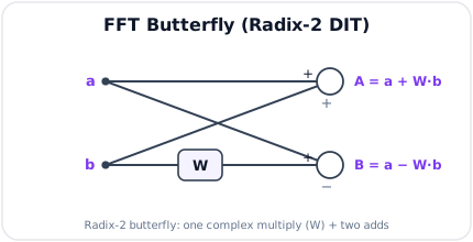
There are \(\log_2N\) stages and \(N/2\) butterflies per stage. Hence a radix-2 FFT requires approximately
instead of approximately \(N^2\) operations for direct evaluation. In a common in-place decimation-in-time implementation, the inputs are arranged in bit-reversed order and the outputs emerge in natural order; bit reversal is an implementation arrangement, not a requirement of every FFT program.
![4-point decimation-in-time FFT flow graph: bit-reversed inputs x[0], x[2], x[1], x[3] pass through two butterfly stages to natural-order outputs X[0..3]](.././img/fft_dit_4point.svg)
Applications
- Spectrum analysis
- OFDM communication systems
- Fast convolution
- Audio and image processing
4. Circular Convolution
Likely Exam Question (10 marks)
"Define circular convolution. How can linear convolution be obtained using DFT?"
Circular Convolution Definition
For two \(N\)-point sequences \(x[n]\) and \(h[n]\), circular convolution is:
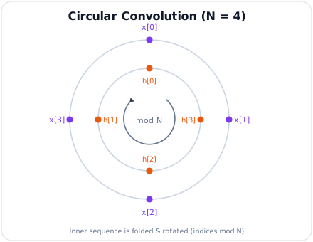
where \((n-m)_N\) means modulo-\(N\) indexing.
Modulo indexing causes samples that would fall beyond \(n=N-1\) to wrap around and add to the beginning of the result. Therefore, circular convolution is the convolution of the periodic extensions of the two \(N\)-point sequences.
DFT Convolution Property
If:
then:
where \(\circledast\) denotes circular convolution.
Linear Convolution Using DFT
To obtain linear convolution of sequences of lengths \(L\) and \(M\) using DFT:
- Choose DFT length \(N \geq L + M - 1\).
- Zero-pad both sequences to length \(N\).
- Compute \(X[k]\) and \(H[k]\).
- Multiply: \(Y[k] = X[k]H[k]\).
- Take IDFT to get linear convolution.
Without sufficient zero-padding, circular convolution causes time-domain aliasing.
If \(y_\ell[n]\) denotes ordinary linear convolution and \(y_c[n]\) denotes an \(N\)-point circular convolution, their precise relation is
The shifted copies of \(y_\ell[n]\) overlap and add every \(N\) samples. This is time-domain aliasing. Choosing \(N\geq L+M-1\) prevents overlap because the complete linear-convolution result then fits within one \(N\)-sample period.
Solved Example - Why Zero-Padding Is Necessary
Let \(x[0]=1\), \(x[1]=2\) and \(h[0]=1\), \(h[1]=1\).
Without padding, their 2-point circular convolution is
so
The ordinary linear convolution is
Indeed, for \(N=2\), the last linear-convolution sample wraps onto the first:
Padding both sequences to \(N=L+M-1=3\) gives \(x=\{1,2,0\}\) and \(h=\{1,1,0\}\). Their 3-point circular convolution is then
Thus zero-padding converts the DFT's inherent circular convolution into the required linear convolution.
5. Parseval's Theorem
Likely Exam Question (5 marks)
"State Parseval's theorem for DFT and explain its meaning."
Statement
For an \(N\)-point DFT pair \(x[n] \leftrightarrow X[k]\):
Meaning
The total energy of a finite sequence can be computed either in the time domain or in the frequency domain. Parseval's theorem is useful for checking DFT calculations and analyzing energy distribution across frequencies.
Energy and Power Spectral Density
Parseval also names where the energy sits in frequency:
- For an energy signal, the energy spectral density (ESD) is \(S_{xx}(\omega)=\lvert X(\omega)\rvert^2\), and the continuous-time Parseval relation is \(\int\lvert x(t)\rvert^2 dt=\frac{1}{2\pi}\int\lvert X(\omega)\rvert^2 d\omega\).
- For a power signal, the power spectral density (PSD) \(S_{xx}(\omega)\) is the Fourier transform of the autocorrelation (the Wiener-Khinchin theorem, Section 6).
Either density gives power (or energy) per unit frequency, so integrating it over all frequencies returns the total power (or energy).
6. Autocorrelation
Likely Exam Question (5 marks)
"Define autocorrelation and state its properties."
Autocorrelation Definition
Autocorrelation measures similarity between a signal and a shifted version of itself.
For a continuous-time energy signal:
For a discrete-time energy signal:
For real signals, complex conjugate can be ignored.
The preceding formulas apply to energy signals. For continuous-time and discrete-time power signals, autocorrelation is defined by time averaging:
For a periodic continuous-time signal, the time average may be taken over any one period:
Properties
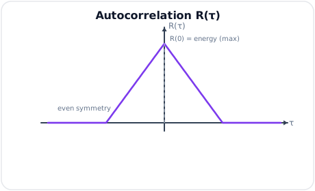
1. Value at Zero
2. Hermitian Symmetry
Hence autocorrelation is real and even for a real-valued signal.
3. Maximum Magnitude at Zero Shift
A signal is most similar to itself when there is no relative delay.
4. Periodicity
If \(x(t)\) is periodic with period \(T_0\), then \(R_{xx}(\tau)\) is also periodic with period \(T_0\).
5. White-Noise Property
Ideal white noise has zero correlation at every non-zero delay:
In discrete time, \(R_{ww}[m]=\sigma_w^2\delta[m]\). This sharp autocorrelation is a property of ideal white noise, not of every random process.
6. Wiener-Khinchin Relation
The Fourier transform of autocorrelation is the energy spectral density or power spectral density:
Cross-Correlation
Cross-correlation measures the similarity between two different signals as one is shifted:
Unlike autocorrelation it is generally not symmetric: \(R_{xy}(\tau)=R_{yx}^*(-\tau)\). Its peak locates the relative delay between \(x\) and \(y\), which is the basis of radar/sonar ranging and receiver synchronization.
Correlation vs Convolution
Correlation is convolution with a time-reversed (and conjugated) signal — the only difference is that convolution folds one signal while correlation does not:
So the same routine (or FFT) that performs convolution also performs correlation once one input is reversed.
Solved Example - Autocorrelation of a Sinusoid
Let \(x(t)=A\cos(\omega_0t+\phi)\), a power signal. Averaging over one period,
At zero delay, \(R_{xx}(0)=A^2/2\), which equals the sinusoid's average power. The correlation is periodic and has peaks at delays equal to integer multiples of the signal period, so autocorrelation can reveal an unknown periodicity even when the signal is noisy.
Uses
- Detecting periodicity
- Measuring similarity and delay
- Radar and sonar signal processing
- Communication synchronization
- Power spectral density analysis
Key Exam Points - Discrete Signal Processing
- DFT converts finite samples into finite frequency bins.
- IDFT reconstructs the time sequence from DFT coefficients.
- FFT is a fast algorithm for DFT, reducing complexity from \(O(N^2)\) to \(O(N\log_2N)\).
- DFT multiplication corresponds to circular convolution.
- Linear convolution using DFT requires zero-padding to \(N \geq L+M-1\).
- Parseval's theorem equates time-domain and frequency-domain energy; ESD \(=\lvert X(\omega)\rvert^2\), PSD \(=\mathcal{F}\{R_{xx}\}\) (Wiener-Khinchin).
- Autocorrelation measures self-similarity vs shift; cross-correlation compares two signals and equals convolution with a folded signal.
Model Answer — DFT, IDFT and Four-Point Example [5–10 marks]
5-mark answer and 10-mark extension
For 5 marks — write this
The \(N\)-point discrete Fourier transform (DFT) converts a finite sequence \(x[n]\), \(0\le n<N\), into \(N\) equally spaced frequency coefficients:
The inverse DFT (IDFT) reconstructs every sample:
The DFT treats the finite record and its spectrum as one period of periodic sequences. If the sampling rate is \(F_s\), bin spacing is \(\Delta f=F_s/N\), and bins above \(N/2\) represent wrapped negative frequencies. For real \(x[n]\), \(X[N-k]=X^*[k]\).
Add for a 10-mark variant
For \(N=4\), \(W_4=e^{-j\pi/2}=-j\) and its powers are \(1,-j,-1,j\). Let
Evaluate each coefficient directly:
Hence
\(X[3]=X^*[1]\) verifies conjugate symmetry. Check the IDFT at \(n=1\):
which recovers the original second sample. The factor \(1/N\) appears only in the IDFT under this convention.
As a separate visual check, the constant sequence \(\{1,1,1,1\}\) transforms to the DC-only result \(\{4,0,0,0\}\):
Important properties are linearity, periodicity \(X[k+N]=X[k]\), circular shift \(x[(n-n_0)_N]\leftrightarrow W_N^{kn_0}X[k]\), and circular convolution \(x\circledast_Nh\leftrightarrow XH\). The DFT is used for sampled-spectrum analysis and fast filtering; it is computed efficiently by the FFT.
Practice target: 9 minutes for definitions or 18 minutes with all four coefficients and one IDFT check; write the twiddle powers before arithmetic.
Model Answer — FFT Computation and Radix-2 DIT Flow [5 marks]
Exam-ready answer
The fast Fourier transform (FFT) is not a new transform; it is an algorithm that computes exactly the \(N\)-point DFT with fewer arithmetic operations. Direct evaluation forms every one of \(N\) outputs from \(N\) input terms, requiring about \(N^2\) complex multiplications and \(N(N-1)\) additions.
For radix-2 decimation in time (DIT), assume \(N=2^r\) and split the DFT into even- and odd-indexed samples. If \(E[k]\) and \(O[k]\) are their \(N/2\)-point DFTs,
These two outputs form one butterfly.
The split is repeated for \(\log_2N\) stages, each containing \(N/2\) butterflies. Consequently,
| Method | Complex multiplications | Order |
|---|---|---|
| Direct DFT | approximately \(N^2\) | \(O(N^2)\) |
| Radix-2 FFT | approximately \((N/2)\log_2N\) | \(O(N\log_2N)\) |
For \(N=1024\), direct evaluation needs about \(1024^2=1,048,576\) multiplications, whereas radix-2 FFT needs \((1024/2)\times10=\boxed{5120}\), a reduction by a factor of about 205.
In a common in-place DIT implementation, input indices are arranged in bit-reversed order and outputs emerge in natural order; there are two stages for \(N=4\). FFT speed makes real-time spectrum analysis, OFDM, fast convolution and correlation practical. The savings come from reusing root-of-unity symmetries such as \(W_N^{k+N/2}=-W_N^k\), not from approximating the DFT.
Practice target: 9 minutes; derive the two butterfly equations, draw one butterfly and compare the operation counts numerically.
Model Answer — Circular and Linear Convolution [5 marks]
Exam-ready answer
For two \(N\)-point sequences, circular convolution is
where \((\cdot)_N\) denotes modulo-\(N\) indexing. The modulo operation wraps samples beyond the last index back to the beginning, because the DFT regards both sequences as periodic.
The DFT convolution theorem is
Ordinary linear convolution of lengths \(L\) and \(M\) has length \(L+M-1\). To obtain it by DFT: choose \(N\ge L+M-1\), append zeros to both sequences to length \(N\), compute their DFTs, multiply bin by bin, and take the IDFT. Without sufficient padding, shifted tails add at the beginning:
which is time-domain aliasing.
Example: for \(x=\{1,2\}\) and \(h=\{1,1\}\), the two-point circular result is
so \(y_c=\{3,3\}\). Linear convolution is \(y_\ell=\{1,3,2\}\). Padding both inputs to \(N=2+2-1=3\) gives the three-point circular result
For long streams, overlap-add and overlap-save divide the data into blocks, use FFT-based circular convolutions with adequate padding, and combine only the unaliased samples. Thus DFT multiplication inherently produces circular convolution; zero-padding is what makes it equal the required linear result.
Practice target: 9 minutes; write the modulo definition, five DFT steps, minimum padding length and both outputs of the two-sample example.
Model Answer — Parseval's Theorem, Signal Energy and Power [5 marks]
Exam-ready answer
For the DFT convention \(X[k]=\sum_{n=0}^{N-1}x[n]e^{-j2\pi kn/N}\), Parseval’s theorem is
It states that total finite-record energy is unchanged by representation; the factor \(1/N\) is required because only the IDFT is normalized. The CT counterpart is
An energy signal has \(0<E<\infty\) and average power \(P=0\); a power signal has \(E=\infty\) and \(0<P<\infty\). For DT signals,
| Type | Example | Result |
|---|---|---|
| Energy | finite pulse | finite \(E\), zero \(P\) |
| Power | nonzero periodic sinusoid | infinite \(E\), finite average \(P\) |
DFT check: for \(x[n]=\{1,1,1,1\}\), \(X[k]=\{4,0,0,0\}\). The time-side energy is \(1+1+1+1=4\), while the frequency side is
Thus Parseval also detects scaling or arithmetic errors in a DFT. For energy signals, \(|X(\omega)|^2\) is energy spectral density. For power signals, power spectral density is obtained from the Fourier transform of autocorrelation by Wiener–Khinchin; integrating the appropriate density returns total energy or average power.
Practice target: 8 minutes; state the DFT normalization, both classifications and verify the theorem with the four-sample constant sequence.
Model Answer — Autocorrelation and Its Properties [5 marks]
Exam-ready answer
Autocorrelation measures similarity between a signal and a delayed copy of itself. For a DT energy signal,
and for a CT energy signal,
For power signals the integral or sum is replaced by a long-time average; this distinction is essential because their total energy diverges.
The principal properties are
and \(R_{xx}[0]=E\) for an energy signal or \(P\) for a power signal. Thus real-signal autocorrelation is real and even and has maximum magnitude at zero lag. If \(x\) is periodic, \(R_{xx}\) has the same period. Ideal DT white noise has \(R_{ww}[m]=\sigma_w^2\delta[m]\).
The Wiener–Khinchin theorem connects correlation and spectrum:
so autocorrelation and power/energy spectral density are a Fourier pair.
Sequence example: let \(x[n]=\{1,2\}\) for \(n=0,1\). Then
and all other lags are zero. Hence \(R_{xx}[m]=\{2,5,2\}\) for \(m=-1,0,1\), confirming even symmetry and the maximum at zero. Correlation is used for delay estimation, radar/sonar ranging, symbol and carrier synchronization, periodicity detection, and spectrum estimation.
Practice target: 9 minutes; distinguish energy and power definitions, list four properties, state Wiener–Khinchin and calculate every nonzero lag of one short sequence.