Transfer Functions and System Response
Possible Exam Questions
Exam Questions and Answer Map
Questions labelled [PYQ paper/year] are observed past questions; those labelled [likely] are pattern-based predictions. For each one, rehearse the answer plan closed-book, then use the links to verify the full answer in this chapter.
-
Define transfer function; state its properties and limitations. [5] — [likely]
-
Answer plan: Define TF as \(C(s)/R(s)\) with zero ICs → state assumptions (LTI, lumped) → list advantages (algebraic, reveals poles/zeros) → list limitations (no initial conditions, SISO only, linear only).
-
Model answer: Transfer-function definition, properties, and limitations
-
Derive the transfer function of a simple closed-loop system (C/R = G/(1+GH)). [5] — [PYQ 2082]
-
Answer plan: Draw basic feedback block diagram → write \(E=R-HC\) → write \(C=GE\) → substitute and solve for \(C/R\) → obtain \(G/(1+GH)\) → state significance of characteristic equation \(1+GH=0\).
-
Model answer: Closed-loop transfer-function derivation
-
Explain poles and zeros; how does their location affect stability and transient response? [4–5] — [PYQ 2082]
-
Answer plan: Define poles (roots of denominator) and zeros (roots of numerator) → tabulate pole-location vs time response (real LHP → decaying exponential, complex LHP → decaying oscillation, RHP → unstable) → explain dominant poles → mention zero effects on overshoot.
-
Model answer: Poles, zeros, stability, and transient response
-
Obtain the transfer function of an electrical (RLC) or mechanical system. [5–10] — [likely]
-
Answer plan: Write KVL/KCL or Newton's law equations → take Laplace transform → rearrange as output/input ratio → identify standard forms (first/second order) → use electrical-mechanical analogy table if needed.
-
Model answer: RLC and mechanical-system transfer functions
-
Derive the transfer function of an armature-controlled DC motor. [10] — [likely]
-
Answer plan: Write armature circuit equation (\(V_a = R_a i_a + L_a di_a/dt + e_b\)) → write back-emf (\(e_b = K_b\omega\)) → write torque equation (\(J\dot\omega + B\omega = K_t i_a\)) → Laplace transform → eliminate \(I_a(s)\) → obtain \(\Omega(s)/V_a(s)\).
- Model answer: Armature-controlled DC motor transfer function
Syllabus Focus
- System transfer functions and responses
- Poles and zeros locations and their significance
- Block diagram reduction
- Signal flow graph and Mason's gain formula
- Time response of first-order and second-order systems
- Steady-state error and error constants
1. Transfer Function
Likely Exam Question (5 marks)
"Define transfer function. State its assumptions, advantages, and limitations."
The transfer function of a linear time-invariant system is the ratio of Laplace transform of output to Laplace transform of input, assuming all initial conditions are zero.
where:
- \(R(s)\) = Laplace transform of input
- \(C(s)\) = Laplace transform of output
- \(s = \sigma + j\omega\)
Assumptions
Transfer function is valid for:
- Linear systems
- Time-invariant systems
- Lumped-parameter systems
- Zero initial conditions
General Form
If a system is described by the differential equation:
Taking Laplace transform with zero initial conditions:
Advantages
- Converts differential equations into algebraic equations.
- Gives direct input-output relation.
- Poles and zeros reveal stability and transient behavior.
- Useful for block diagram and frequency-response analysis.
- Independent of input signal.
Limitations
- Does not apply directly to nonlinear systems.
- Does not include initial condition effects.
- Gives no internal state information.
- Different physical systems can have the same transfer function.
- Mainly suitable for SISO systems.
2. Poles and Zeros
Likely Exam Question (10 marks)
"Define poles and zeros. Explain the significance of pole-zero locations in control-system response."
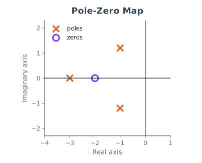
For a transfer function:
Zeros
Zeros are the roots of numerator \(N(s)\).
At a zero, the transfer function becomes zero.
Poles
Poles are the roots of denominator \(D(s)\).
At a pole, the transfer function becomes infinite.
Example
Zero: \(s=-2\)
Poles: \(s=-2,-3\)
If the common factor is physically cancelled, the reduced transfer function is:
However, exact pole-zero cancellation is risky in real systems because model uncertainty can leave hidden unstable modes.
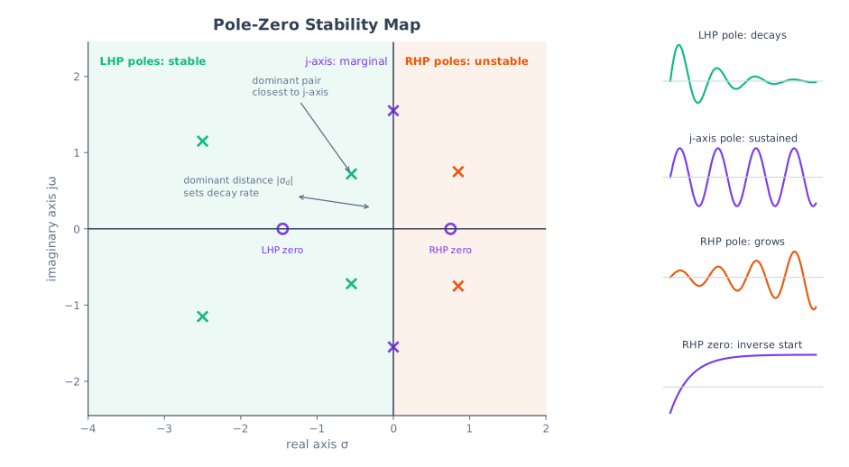
Significance of Pole Locations
| Pole Location | Time Response | Stability |
|---|---|---|
| Negative real axis | Decaying exponential | Stable |
| Positive real axis | Growing exponential | Unstable |
| Origin | Constant or ramp component | Marginal/integrating behavior |
| Imaginary axis | Sustained oscillation | Marginal if simple |
| Complex LHP | Decaying oscillation | Stable |
| Complex RHP | Growing oscillation | Unstable |
Dominant Poles
Dominant poles are poles closest to the imaginary axis. They decay most slowly and dominate transient response.
For stable systems:
- Poles far left decay quickly.
- Poles near imaginary axis decay slowly.
- Dominant complex poles mainly determine overshoot and settling time.
Significance of Zeros
Zeros shape transient response and frequency response.
Effects of zeros:
- Can increase overshoot.
- Can speed up response.
- Can introduce undershoot if located in right half-plane.
- Can partially cancel pole effects.
Right-half-plane zeros are called non-minimum phase zeros and cause inverse response, making control more difficult.
3. Mathematical Modeling of Physical Systems
Likely Exam Question (10 marks)
"Derive the transfer function of a mechanical translational system or an RLC electrical network."
Electrical System Elements
| Element | Time-Domain Relation | Impedance in \(s\)-Domain |
|---|---|---|
| Resistor \(R\) | \(v=Ri\) | \(R\) |
| Inductor \(L\) | \(v=L\frac{di}{dt}\) | \(Ls\) |
| Capacitor \(C\) | \(i=C\frac{dv}{dt}\) | \(1/(Cs)\) |
Mechanical Translational Elements
| Element | Force Relation | Mechanical Impedance |
|---|---|---|
| Mass \(M\) | \(F=M\frac{d^2x}{dt^2}\) | \(Ms^2\) for displacement relation |
| Damper \(B\) | \(F=B\frac{dx}{dt}\) | \(Bs\) |
| Spring \(K\) | \(F=Kx\) | \(K\) |
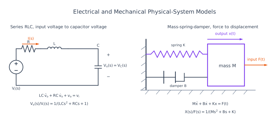
For a mass-spring-damper system:
Taking Laplace transform:
Transfer function from force to displacement:
Rotational Mechanical Elements
| Element | Torque Relation |
|---|---|
| Moment of inertia \(J\) | \(T=J\frac{d^2\theta}{dt^2}\) |
| Viscous friction \(B\) | \(T=B\frac{d\theta}{dt}\) |
| Torsional spring \(K\) | \(T=K\theta\) |
For rotational system:
Electrical-Mechanical Analogies
| Force-Voltage Analogy | Force-Current Analogy |
|---|---|
| Force \(F\) analogous to voltage \(V\) | Force \(F\) analogous to current \(I\) |
| Velocity \(v\) analogous to current \(i\) | Velocity \(v\) analogous to voltage \(V\) |
| Mass \(M\) analogous to inductance \(L\) | Mass \(M\) analogous to capacitance \(C\) |
| Damper \(B\) analogous to resistance \(R\) | Damper \(B\) analogous to conductance \(1/R\) |
| Spring \(K\) analogous to inverse capacitance \(1/C\) | Spring \(K\) analogous to inverse inductance \(1/L\) |
4. DC Motor Transfer Function
Likely Exam Question (10 marks)
"Derive the transfer function of an armature-controlled DC motor."
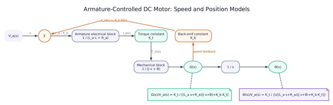
For an armature-controlled DC motor:
Electrical equation:
Back emf:
Torque:
Mechanical equation:
Taking Laplace transform:
Eliminate \(I_a(s)\):
Therefore speed transfer function is:
Since \(\Omega(s)=s\Theta(s)\), position transfer function is:
If armature inductance is negligible, \(L_a \approx 0\):
5. Block Diagram Reduction
Likely Exam Question (10 marks)
"Reduce a block diagram to obtain the overall transfer function. State the rules of block diagram reduction."
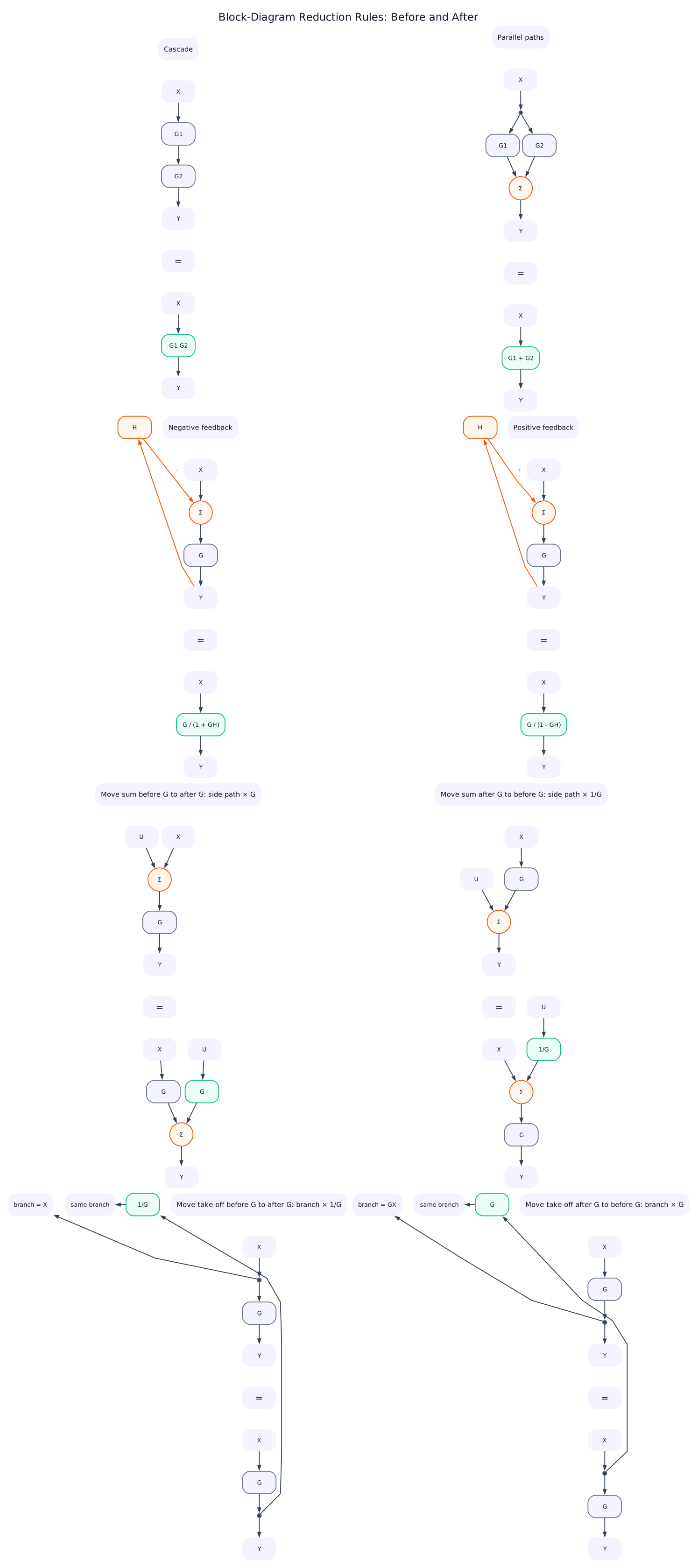
A block diagram represents a system using functional blocks and signal-flow directions.
Basic Rules
| Connection | Equivalent Transfer Function |
|---|---|
| Cascade blocks | \(G_1G_2\) |
| Parallel blocks | \(G_1+G_2\) |
| Negative feedback | \(G/(1+GH)\) |
| Positive feedback | \(G/(1-GH)\) |
Moving Summing Point
When moving a summing point before or after a block, insert the proper compensating block so the signal remains unchanged.
If a summing point is moved from after \(G\) to before \(G\), the side input must be multiplied by \(1/G\).
If a summing point is moved from before \(G\) to after \(G\), the side input must be multiplied by \(G\).
Moving Take-Off Point
If a take-off point is moved from before \(G\) to after \(G\), insert \(1/G\) in the branch.
If a take-off point is moved from after \(G\) to before \(G\), insert \(G\) in the branch.
Reduction Strategy
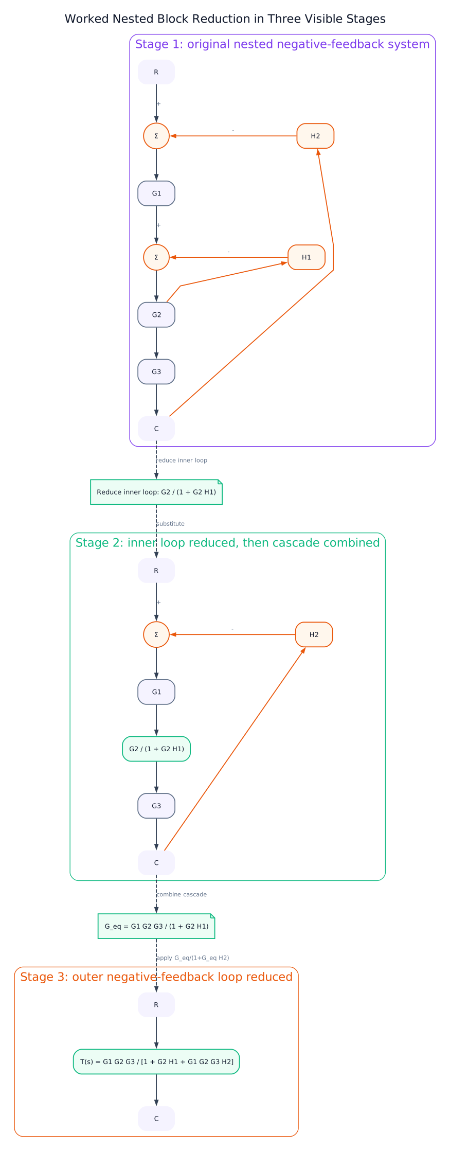
- Combine cascade blocks.
- Combine parallel blocks.
- Reduce inner feedback loops first.
- Move summing/take-off points only when necessary.
- Continue until a single equivalent block remains.
6. Signal Flow Graph
Likely Exam Question (10 marks)
"State Mason's gain formula and use it to find the transfer function of a signal flow graph."
A signal flow graph is a graphical representation of linear algebraic equations using nodes and directed branches.
Terms
| Term | Meaning |
|---|---|
| Node | Variable or signal |
| Branch | Directed path from one node to another |
| Branch gain | Gain/transmittance of a branch |
| Input node/source | Node with only outgoing branches |
| Output node/sink | Node with only incoming branches |
| Forward path | Path from input to output without repeating a node |
| Loop | Closed path starting and ending at same node without repeating another node |
| Non-touching loops | Loops that do not share any node |
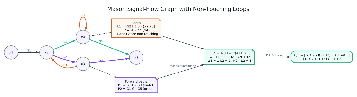
Mason's Gain Formula
Overall transfer function is:
where:
- \(P_k\) = gain of \(k\)th forward path
- \(\Delta\) = graph determinant
- \(\Delta_k\) = value of \(\Delta\) excluding loops that touch the \(k\)th forward path
Graph determinant:
Steps
- Identify all forward paths and their gains.
- Identify all individual loops and loop gains.
- Identify non-touching loop combinations.
- Compute \(\Delta\).
- Compute each \(\Delta_k\).
- Apply Mason's formula.
7. Standard Test Signals
Likely Exam Question (5 marks)
"Why are standard test inputs used in control systems? Give their Laplace transforms."
Standard test signals are used to compare system performance under common inputs.
| Input | Time Function | Laplace Transform |
|---|---|---|
| Unit impulse | \(\delta(t)\) | \(1\) |
| Unit step | \(u(t)\) | \(1/s\) |
| Unit ramp | \(t\,u(t)\) | \(1/s^2\) |
| Unit parabolic | \(\frac{t^2}{2}u(t)\) | \(1/s^3\) |
| Sinusoidal | \(\sin\omega t\) | \(\omega/(s^2+\omega^2)\) |
Step input tests set-point regulation, ramp input tests tracking of constant-velocity commands, and parabolic input tests constant-acceleration tracking.
8. First-Order System Response
Likely Exam Question (5 marks)
"Derive the unit-step response of a first-order system and define time constant."
Standard first-order transfer function:
where \(T\) is the time constant.
Unit-Step Response
For unit step input:
Taking inverse Laplace:
Important Values
| Time | Response |
|---|---|
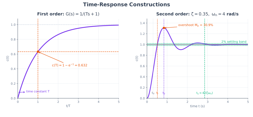
| \(t=T\) | \(c(T)=1-e^{-1}=0.632\) or 63.2% |
| \(t=2T\) | 86.5% |
| \(t=3T\) | 95% |
| \(t=4T\) | 98.2% |
| \(t=5T\) | 99.3% |
Specifications
For first-order system:
9. Second-Order System Response
Likely Exam Question (10 marks)
"For a standard second-order system, define damping ratio, natural frequency, peak overshoot, rise time, peak time, and settling time."
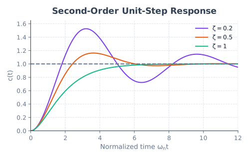
Standard second-order closed-loop transfer function:
where:
- \(\omega_n\) = undamped natural frequency
- \(\zeta\) = damping ratio
Characteristic equation:
Poles:
For \(0<\zeta<1\), define damped natural frequency:
Damping Cases
| Damping Ratio | Poles | Response |
|---|---|---|
| \(\zeta=0\) | Pure imaginary | Undamped oscillation |
| \(0<\zeta<1\) | Complex LHP | Underdamped oscillation with decay |
| \(\zeta=1\) | Equal real poles | Critically damped, fastest non-oscillatory |
| \(\zeta>1\) | Distinct real poles | Overdamped, slow non-oscillatory |
| \(\zeta<0\) | RHP poles | Unstable |
Unit-Step Response for Underdamped System
For \(0<\zeta<1\):
where:
Time-Domain Specifications
| Specification | Symbol | Formula |
|---|---|---|
| Delay time | \(t_d\) | Time to reach 50% of final value |
| Rise time | \(t_r\) | Time to rise from 0% to 100% for underdamped system |
| Peak time | \(t_p\) | \(\frac{\pi}{\omega_d}\) |
| Maximum overshoot | \(M_p\) | \(e^{-\pi\zeta/\sqrt{1-\zeta^2}}\) |
| Percent overshoot | \(\%OS\) | \(100e^{-\pi\zeta/\sqrt{1-\zeta^2}}\) |
| Settling time, 2% criterion | \(t_s\) | \(\frac{4}{\zeta\omega_n}\) |
| Settling time, 5% criterion | \(t_s\) | \(\frac{3}{\zeta\omega_n}\) |
Approximate rise time for underdamped system:
Effect of \(\zeta\) and \(\omega_n\)
- Increasing \(\zeta\) reduces overshoot but may slow response.
- Increasing \(\omega_n\) generally speeds up response.
- Larger \(\zeta\omega_n\) gives faster decay and smaller settling time.
- Dominant poles farther left in the \(s\)-plane give faster settling.
10. Steady-State Error
Likely Exam Question (10 marks)
"Define position, velocity, and acceleration error constants. Find steady-state error for step, ramp, and parabolic inputs."
Steady-state error is the difference between input and output as \(t\to\infty\).
Using final value theorem:
For a unity-feedback system:
Therefore:
Static Error Constants
For unity feedback:
| Error Constant | Definition | Input |
|---|---|---|
| Position error constant | \(K_p=\lim_{s\to0}G(s)\) | Step |
| Velocity error constant | \(K_v=\lim_{s\to0}sG(s)\) | Ramp |
| Acceleration error constant | \(K_a=\lim_{s\to0}s^2G(s)\) | Parabolic |
Steady-State Error Formulas
| Input | \(R(s)\) | Steady-State Error |
|---|---|---|
| Unit step | \(1/s\) | \(e_{ss}=\frac{1}{1+K_p}\) |
| Unit ramp | \(1/s^2\) | \(e_{ss}=\frac{1}{K_v}\) |
| Unit parabolic | \(1/s^3\) | \(e_{ss}=\frac{1}{K_a}\) |
System Type
System type is the number of pure integrators, or poles at origin, in the open-loop transfer function \(G(s)H(s)\).
| System Type | Poles at Origin | Step Error | Ramp Error | Parabolic Error |
|---|---|---|---|---|
| Type 0 | 0 | finite | \(\infty\) | \(\infty\) |
| Type 1 | 1 | 0 | finite | \(\infty\) |
| Type 2 | 2 | 0 | 0 | finite |
Important:
- Increasing system type improves steady-state accuracy.
- Adding integrators reduces steady-state error but may reduce stability.
11. Solved Examples
Example 1 - Transfer Function from Differential Equation
Q. Find transfer function if:
Solution:
Taking Laplace transform with zero initial conditions:
Example 2 - Poles, Zeros, and Stability
Q. Find poles and zeros of \(G(s)=\frac{5(s+4)}{s(s+2)(s^2+2s+5)}\) and comment on stability.
Solution:
Zero: \(s=-4\)
Poles:
All poles are in left half-plane except one pole at origin. Therefore the system is marginal/integrating in open-loop sense. Closed-loop stability must be checked from closed-loop characteristic equation.
Example 3 - Second-Order Specifications
Q. A standard second-order system has \(\zeta=0.5\) and \(\omega_n=10\,\text{rad/s}\). Find \(\omega_d\), \(t_p\), percent overshoot, and 2% settling time.
Solution:
Example 4 - Steady-State Error
Q. For unity feedback system \(G(s)=\frac{10}{s(s+2)}\), find error constants and steady-state errors for unit step and unit ramp inputs.
Solution:
System has one pole at origin, so it is Type 1.
12. Quick Revision Table
| Topic | Key Result |
|---|---|
| Transfer function | \(G(s)=C(s)/R(s)\) with zero initial conditions |
| Pole | Root of denominator |
| Zero | Root of numerator |
| Stable pole region | Left half of \(s\)-plane |
| Mass-spring-damper | \(X(s)/F(s)=1/(Ms^2+Bs+K)\) |
| DC motor speed TF | \(\Omega(s)/V_a(s)=K_t/[(L_as+R_a)(Js+B)+K_bK_t]\) |
| Cascade blocks | \(G_1G_2\) |
| Parallel blocks | \(G_1+G_2\) |
| Negative feedback | \(G/(1+GH)\) |
| Mason formula | \(T=\sum P_k\Delta_k/\Delta\) |
| First-order step response | \(c(t)=1-e^{-t/T}\) |
| Second-order transfer function | \(\omega_n^2/(s^2+2\zeta\omega_ns+\omega_n^2)\) |
| Peak time | \(t_p=\pi/\omega_d\) |
| Percent overshoot | \(100e^{-\pi\zeta/\sqrt{1-\zeta^2}}\) |
| 2% settling time | \(t_s=4/(\zeta\omega_n)\) |
| Position error constant | \(K_p=\lim_{s\to0}G(s)\) |
| Velocity error constant | \(K_v=\lim_{s\to0}sG(s)\) |
| Acceleration error constant | \(K_a=\lim_{s\to0}s^2G(s)\) |
Key Exam Points - Transfer Functions and Response
- Transfer function is defined only for zero initial conditions.
- Poles decide natural response and stability; zeros shape transient response.
- Dominant poles closest to the imaginary axis control transient behavior.
- Standard second-order formulas are frequently asked in numerical problems.
- System type decides steady-state error for step, ramp, and parabolic inputs.
Model Answer — Transfer-Function Definition, Properties, and Limitations [5 marks]
Exam-ready answer
For a lumped, linear time-invariant system, the transfer function is the ratio of the Laplace transform of output to input with every independent initial condition set to zero:
Input and output reference directions must be declared; reversing either direction changes the corresponding sign. The units of \(G\) are output units divided by input units, for example \((\text{rad/s})/\text{V}\) for a motor speed plant.
If an LTI differential equation is
its zero-state Laplace transform gives
The roots \(z_i\) are zeros and \(p_k\) are poles. Important properties are: \(G\) describes system dynamics independently of a particular input; cascade blocks multiply, parallel blocks add, and a negative-feedback loop reduces to \(G/(1+GH)\); the impulse response is \(g(t)=\mathcal L^{-1}\{G(s)\}\); poles determine natural modes and stability, while zeros shape forced response. Frequency response follows by evaluating \(G(j\omega)\) when the imaginary axis is in the region of convergence.
Worked derivation: for \(\tau\dot c+c=Kr\) with \(\tau>0\) s, zero initial conditions give \((\tau s+1)C=KR\), hence
A unit step produces \(c(t)=K(1-e^{-t/\tau})u(t)\); at \(t=\tau\), it reaches \(0.632K\), checking the pole \(-1/\tau\).
Advantages: differential equations become algebraic; interconnections, steady state, transients, poles/zeros and frequency response are handled systematically. Limitations: a transfer function omits nonzero initial-state response, is not directly valid for nonlinear or time-varying systems, and a scalar form does not capture MIMO interactions or internal state structure. Pole-zero cancellation can hide an unstable internal mode, and parameter uncertainty, saturation and delay must be modeled explicitly. State-space or nonlinear models are used when these limitations matter.
Practice target: 9 minutes; derive the polynomial ratio from a differential equation and separate properties from modeling limitations.
Model Answer — Closed-Loop Transfer-Function Derivation [5 marks]
Exam-ready answer
Assume an LTI SISO system with zero initial conditions. At the negative-feedback summing junction, define the reference as positive and the feedback signal as negative:
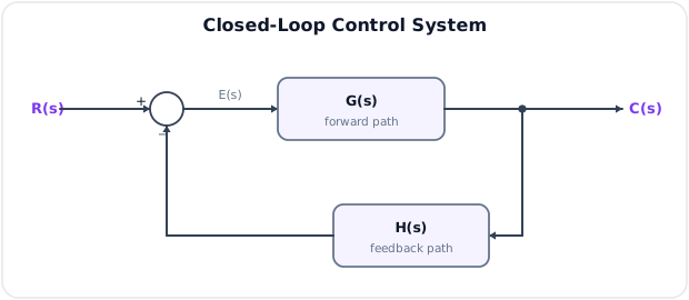
Substitution and collection of the output terms give
The product \(L(s)=G(s)H(s)\) is loop transfer. The characteristic equation
sets the closed-loop poles and therefore stability and natural response. If the summing sign were positive, the denominator would be \(1-GH\); the sign must come from the diagram, not memory.
The same result follows from standard block reduction: a single negative-feedback loop around forward block \(G\) reduces to \(G/(1+GH)\).
It also follows from Mason's gain formula. In the signal-flow graph, the forward path is \(P_1=G\) and the loop gain is \(L_1=-GH\); hence \(\Delta=1-L_1=1+GH\), \(\Delta_1=1\), and \(T=P_1\Delta_1/\Delta=G/(1+GH)\). For larger graphs,
where \(\Delta\) contains loop and non-touching-loop products.
Check: with \(G=10/(s+2)\) and unity feedback, \(T=10/(s+12)\). The pole moves from \(-2\) to \(-12\), DC gain changes from \(5\) to \(10/12\), and the first-order response becomes faster. Reduction and Mason analysis assume linear signal relations; nonlinear saturation or a moved summing/take-off point without the required compensating block invalidates the algebra.
Practice target: 9 minutes; derive from signal equations first, then identify the characteristic equation and one independent reduction check.
Model Answer — Poles, Zeros, Stability, and Transient Response [5 marks]
Exam-ready answer
Write a proper rational transfer function as
A zero \(z_i\) makes the numerator zero and blocks or reshapes response at that complex frequency. A pole \(p_k\) makes the denominator zero and corresponds to a natural mode \(e^{p_kt}\). The horizontal coordinate \(\sigma=\operatorname{Re}s\) has units s\(^{-1}\) and sets exponential growth/decay; the vertical coordinate \(\omega=\operatorname{Im}s\) is oscillation frequency in rad/s.
| Pole location | Natural response and implication |
|---|---|
| Real LHP, \(p=-a\) | \(e^{-at}\): nonoscillatory decay; farther left is faster |
| Complex LHP, \(-\sigma\pm j\omega_d\) | Decaying oscillation; damping set by \(\sigma\) |
| Simple imaginary-axis pair | Sustained natural oscillation; marginal internally, not strict BIBO stability |
| Any RHP pole | Growing exponential/oscillation: unstable |
| Repeated imaginary-axis pole | Polynomially growing oscillation: unstable |
For a standard second-order denominator,
Poles nearest the imaginary axis generally dominate the long transient. For \(0<\zeta<1\), \(t_s\approx4/(\zeta\omega_n)\) s for the 2% criterion and \(M_p=e^{-\pi\zeta/\sqrt{1-\zeta^2}}\).
Zeros do not set asymptotic stability but alter rise, overshoot and phase. A nearby LHP zero can speed response and increase overshoot; a RHP zero causes nonminimum-phase behavior, often an initial motion opposite the final value and a bandwidth limitation. Exact cancellation is unsafe: uncertainty leaves a residual mode, and cancelling an unstable pole can hide internal instability.
Check: \(s^2+4s+25\) has \(\omega_n=5\) rad/s, \(\zeta=0.4\), and poles \(-2\pm j4.58\), so it is stable and underdamped. The approximations give \(t_s\approx2\) s and \(M_p\approx25.4\%\). A zero at \(+1\) would not move those poles but would introduce inverse response. These ideas support controller design, model reduction and transient prediction, subject to the accuracy of the pole-zero model.
Practice target: 9 minutes; mark pole regions on an s-plane and connect each location to its time-domain mode before discussing zeros.
Model Answer — RLC and Mechanical-System Transfer Functions [10 marks]
Exam-ready answer
A physical transfer function is obtained by choosing positive input/output directions, writing conservation laws with passive signs, applying the Laplace transform with zero initial conditions, and forming output over input.
Series RLC system. Let current \(i(t)\) flow from the positive terminal of input voltage \(v_i(t)\) through \(R\), \(L\) and \(C\), and let capacitor voltage \(v_c(t)\) be positive at the current-entering plate. KVL gives
Substituting current,
With zero capacitor voltage and inductor current initially,
and therefore
Here \(R\) is in ohms, \(L\) in henries, \(C\) in farads and the voltage ratio is dimensionless. Comparing with \(\omega_n^2/(s^2+2\zeta\omega_ns+\omega_n^2)\) gives
Translational mechanical system. Let positive displacement \(x(t)\) and applied force \(F(t)\) point to the right. The spring, viscous damper and inertia oppose positive motion with forces \(-Kx\), \(-B\dot x\) and \(-M\ddot x\). Newton's law gives
Under zero initial displacement and velocity,
Here \(M\) is kg, \(B\) is N·s/m, \(K\) is N/m, and \(X/F\) is m/N. The natural parameters are
Using charge \(q\) for the series circuit, \(L\ddot q+R\dot q+q/C=v_i\), which has the force-voltage analogy \(L\leftrightarrow M\), \(R\leftrightarrow B\), \(1/C\leftrightarrow K\), \(q\leftrightarrow x\), and \(v_i\leftrightarrow F\).
Worked check: for \(R=2\,\Omega\), \(L=0.5\) H and \(C=0.1\) F,
Thus \(\omega_n=\sqrt{20}=4.47\) rad/s and \(\zeta=4/(2\sqrt{20})=0.447\); the DC gain is one, consistent with the capacitor becoming open circuit at steady DC. Both models are second order because two independent energy-storage mechanisms exist: electric/magnetic energy in \(C,L\), and kinetic/elastic energy in \(M,K\).
The RLC model applies to filters and resonant networks; the mechanical model applies to suspensions, instruments and servo loads. Ideal lumped, linear elements omit parasitics, Coulomb friction, backlash, saturation and distributed modes. Nonzero initial energy adds separate response terms and is not part of the transfer function.
Practice target: 18–20 minutes; state signs before KVL/Newton equations, derive both ratios, and compare their natural frequency and damping.
Model Answer — Armature-Controlled DC Motor Transfer Function [10 marks]
Exam-ready answer
Consider a separately excited armature-controlled DC motor with constant field flux. Choose positive armature voltage \(v_a\), current \(i_a\), electromagnetic torque and angular speed \(\omega\) in the same motoring sense. Back emf opposes the applied voltage, and positive load torque \(T_L\) opposes rotation. The linear relations are
Here \(R_a\) is in \(\Omega\), \(L_a\) in H, \(K_b\) in V·s/rad, \(K_t\) in N·m/A, \(J\) in kg·m\(^2\), \(B\) in N·m·s/rad, \(\omega\) in rad/s and torque in N·m. Neglecting initial current and speed, the Laplace equations are
For the voltage-to-speed transfer set \(T_L=0\). From the mechanical equation,
Substitute into the electrical equation:
Therefore
Since \(\Omega=s\Theta\) under zero initial position,
The term \(K_tK_b\) is electromechanical negative feedback: increased speed raises opposing back emf, reducing current and torque. Retaining load torque and setting \(V_a=0\) gives the signed disturbance transfer
where the minus sign follows from the declared opposing \(T_L\) direction.
Worked check: take \(R_a=2\,\Omega\), \(L_a=0.5\) H, \(J=0.02\) kg·m\(^2\), \(B=0.10\) N·m·s/rad, and \(K_t=K_b=0.10\) in SI units. Then
The DC speed gain is \(0.10/0.21=0.476\) (rad/s)/V; substitution into the steady electrical and mechanical equations gives the same value.
The model supports speed/position servo design, drive simulation and disturbance analysis. It assumes constant field, linear magnetic circuit, viscous friction and rigid inertia; armature reaction, saturation, Coulomb friction, backlash, converter delay and load elasticity require extensions. If \(L_a\) is negligible relative to the mechanical time scale, the speed model may be approximated as first order, but that approximation must be justified.
Practice target: 18–20 minutes; declare torque signs, eliminate armature current step by step, and include both speed and position forms plus the load-torque check.