Analog Filters
Possible Exam Questions
Exam Questions and Answer Map
Questions marked [PYQ paper/year] were directly observed in past papers; [likely] means pattern-based prediction, not a claimed past question. Rehearse each answer plan closed-book, then check the full answer via the links.
-
Compare Butterworth and Chebyshev filters. [5] — [likely]
-
Answer plan: Contrast flatness, ripple, roll-off, required order and phase response → write both magnitude-response equations.
-
Model answer: Butterworth and Chebyshev Filter Comparison
-
Explain a first-order active Butterworth low-pass filter. [10] — [likely]
-
Answer plan: State the active-filter advantages → write \(H(s)=1/(1+sRC)\) and \(f_c=1/(2pi RC)\) → explain the −3 dB cutoff and −20 dB/decade roll-off.
-
Model answer: First-Order Active Butterworth Low-Pass Filter
-
Determine the order of a Butterworth filter from passband and stopband specifications. [5] — [likely]
-
Answer plan: State \(A_p\), \(A_s\), \(omega_p\) and \(omega_s\) → substitute in the order inequality → round up to the next integer.
- Model answer: Butterworth Filter Order from Specifications
1. Analog Filters — Butterworth and Chebyshev
Likely Exam Question (10 marks)
"Compare Butterworth and Chebyshev filters. Derive the transfer function of a first-order Butterworth low-pass filter." OR "What is a maximally flat response? Why is it called Butterworth?"
Analog Filters — Overview
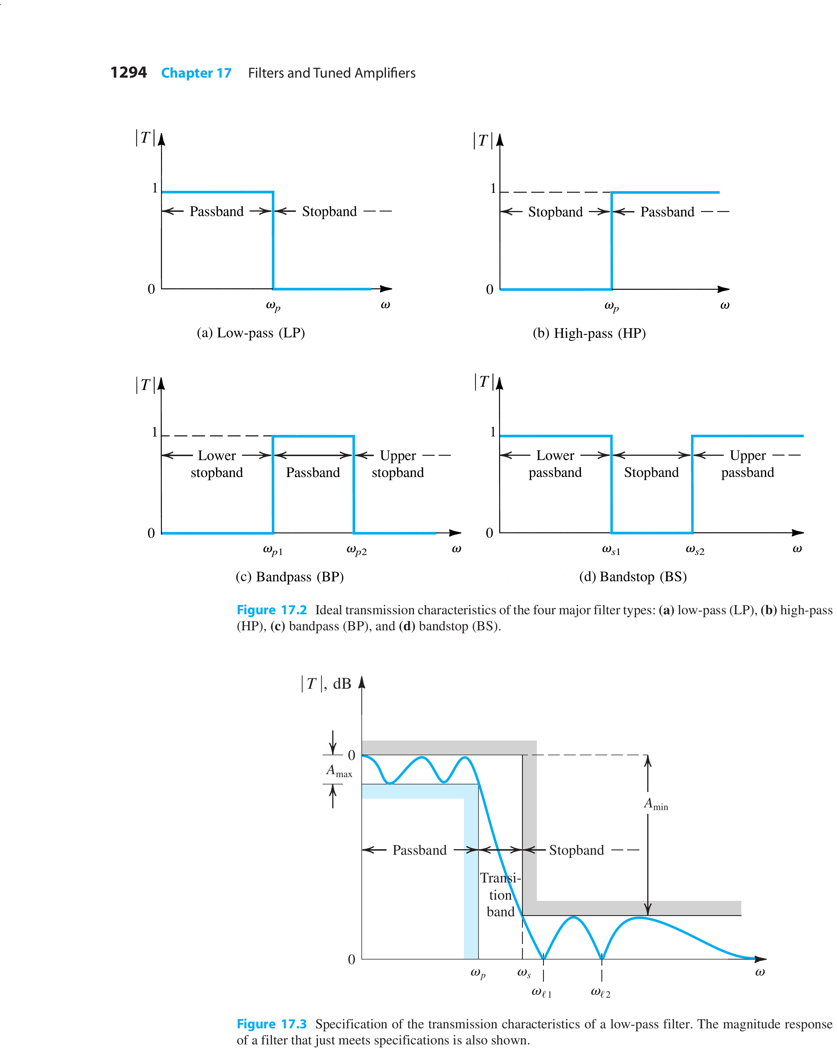
An analog filter is a circuit that selectively passes signals within a certain frequency range (passband) while attenuating signals outside that range (stopband). The transition between passband and stopband is characterised by the filter's order — higher order → sharper transition.
Filter types by frequency response:
- Low-pass: Passes frequencies below cutoff \(f_c\).
- High-pass: Passes frequencies above cutoff \(f_c\).
- Band-pass: Passes frequencies between \(f_L\) and \(f_H\).
- Band-stop (notch): Rejects frequencies between \(f_L\) and \(f_H\).
Butterworth Filter
Definition: The Butterworth filter (also called a maximally flat magnitude filter) is an analog filter designed so that the frequency response in the passband is as flat as possible — there are no ripples in the passband. It provides the best Taylor series approximation to the ideal "brick wall" response at \(\omega = 0\).
Magnitude-squared response:
where \(n\) is the filter order and \(\omega_c\) is the cutoff frequency (–3 dB frequency).
Key properties:
- Maximally flat passband: All derivatives of the magnitude up to order \((2n-1)\) are zero at \(\omega = 0\).
- At \(\omega = \omega_c\): \(|H(j\omega_c)|^2 = 1/2\) → magnitude = \(1/\sqrt{2}\) → gain = –3 dB.
- Roll-off rate: \(-20n\) dB/decade in the stopband (–20 dB/decade per order).
- No passband ripple, no stopband ripple (monotonic response).
- Phase response is nonlinear (not constant group delay).
Transfer function — First-order Butterworth LPF (\(n=1\)):
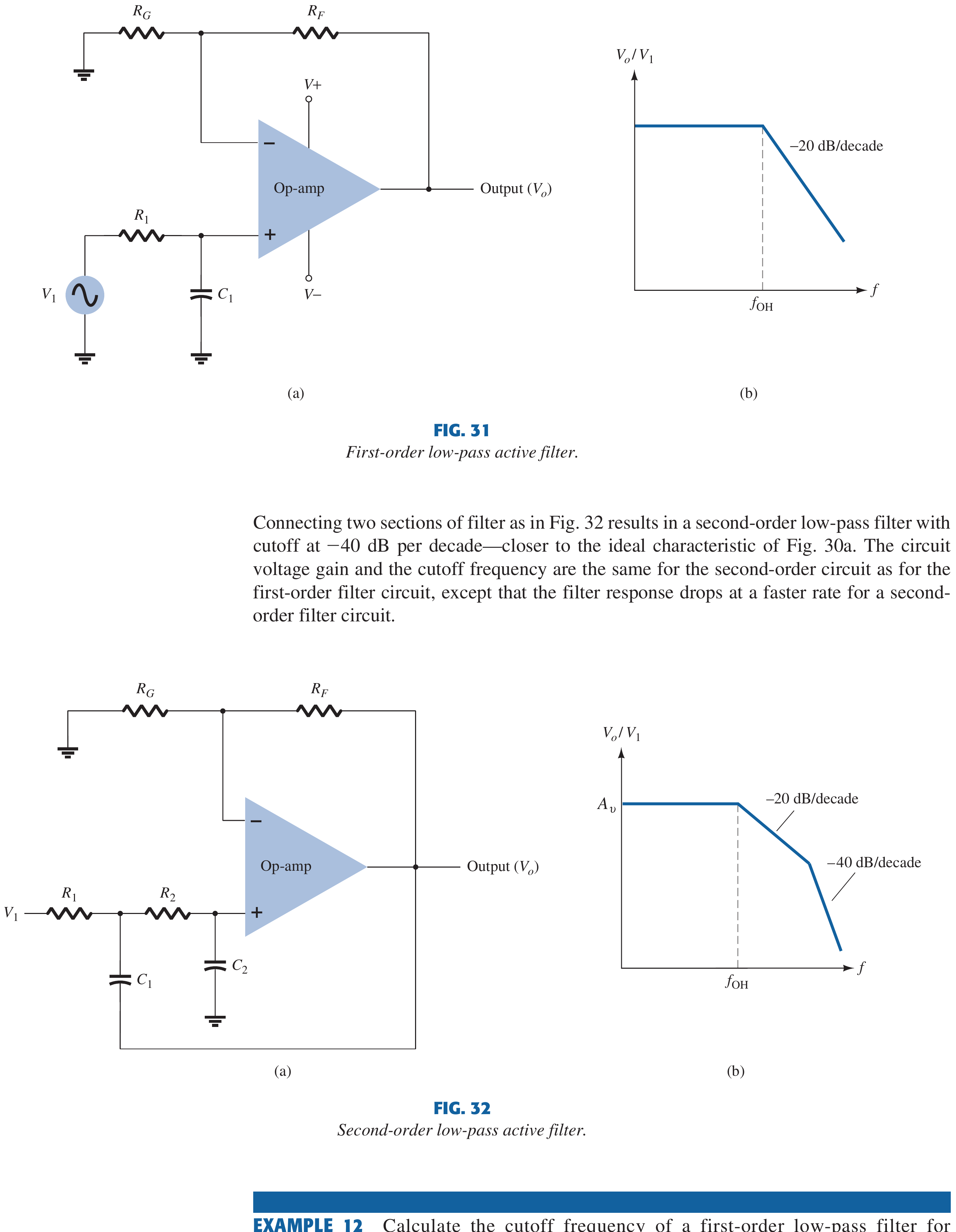
Active implementation (using op-amp): A first-order Butterworth LPF uses one op-amp with a single RC network:
First- and Second-Order High-Pass Active Filters
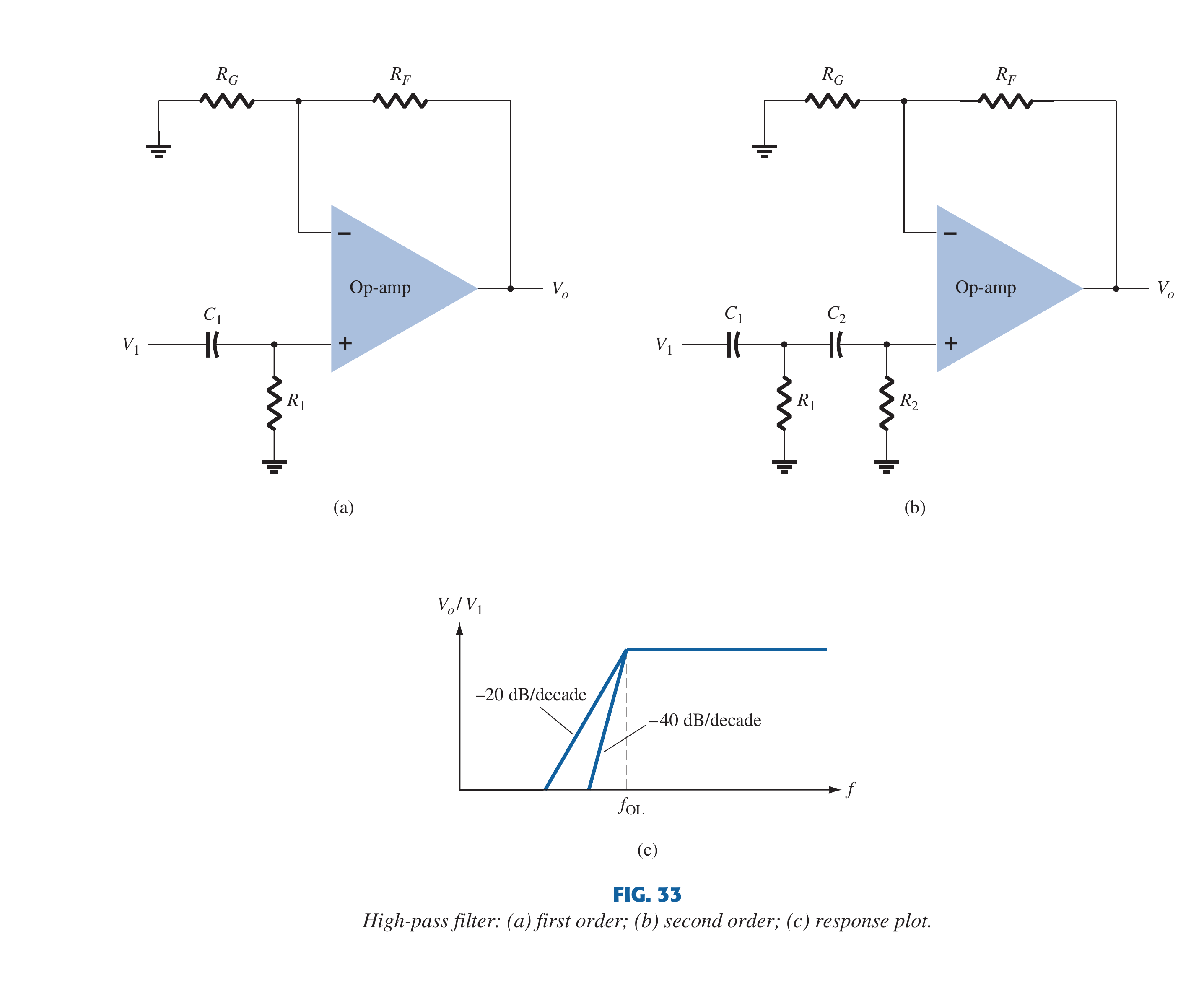
- A first-order high-pass section has \(f_c=1/(2\pi RC)\) and rises at 20 dB/decade below cutoff.
- A second-order section uses two reactive poles and rises at 40 dB/decade below cutoff; its damping (or \(Q\)) depends on component ratios and closed-loop gain.
- Above the passband edge, the non-inverting op-amp sets the finite gain; the capacitor network blocks DC.
Source figure: Boylestad/Nashelsky, Electronic Devices and Circuit Theory (11th ed.), PDF p. 694.
Transfer function — Second-order Butterworth LPF (\(n=2\)):
The denominator polynomial is the 2nd-order Butterworth polynomial: \(s^2 + \sqrt{2}\,\omega_c s + \omega_c^2\). The damping ratio \(\zeta = 1/\sqrt{2} \approx 0.707\), quality factor \(Q = 1/\sqrt{2} \approx 0.707\).
\(n\)th-order Butterworth poles: The \(2n\) poles of \(|H(s)|^2\) lie equally spaced on a circle of radius \(\omega_c\) in the \(s\)-plane. The stable poles (left-half plane) are selected for \(H(s)\):
Determining filter order: Given passband attenuation \(A_p\) at \(\omega_p\) and stopband attenuation \(A_s\) at \(\omega_s\):
Chebyshev Filter
Definition: The Chebyshev filter (Type I) achieves a sharper roll-off (faster transition from passband to stopband) than a Butterworth filter of the same order, at the cost of introducing equi-ripple (equal-amplitude oscillations) in the passband.
Magnitude-squared response (Type I):
where:
- \(T_n\) is the Chebyshev polynomial of degree \(n\)
- \(\varepsilon\) is the ripple parameter (controls passband ripple amplitude)
- Passband ripple in dB: \(R_p = 10 \log_{10}(1 + \varepsilon^2)\)
Chebyshev polynomials:
- \(T_0(x) = 1\)
- \(T_1(x) = x\)
- \(T_2(x) = 2x^2 - 1\)
- \(T_3(x) = 4x^3 - 3x\)
- Recursion: \(T_{n+1}(x) = 2x \cdot T_n(x) - T_{n-1}(x)\)
Key properties:
- Equi-ripple passband: The magnitude oscillates between \(1\) and \(1/\sqrt{1+\varepsilon^2}\) in the passband. All ripple peaks have the same amplitude (equi-ripple).
- Sharper roll-off than Butterworth for the same order \(n\).
- Monotonic stopband (no ripple in stopband — this is Type I; Type II has stopband ripple instead).
- Worse phase response (more nonlinear) than Butterworth.
Type II Chebyshev (Inverse Chebyshev):
- Flat passband (no passband ripple), equi-ripple in stopband.
- Less commonly used.
Butterworth vs Chebyshev — Comparison
| Feature | Butterworth | Chebyshev (Type I) |
|---|---|---|
| Passband response | Maximally flat (no ripple) | Equi-ripple (oscillations) |
| Stopband response | Monotonic | Monotonic |
| Roll-off rate | Moderate (\(-20n\) dB/decade) | Sharper (steeper for same \(n\)) |
| Required order | Higher order needed for sharp cutoff | Lower order achieves same sharpness |
| Phase response | Moderately nonlinear | More nonlinear (worse) |
| Group delay | Approximately constant | Less constant (more distortion) |
| Design complexity | Simpler | More complex (ripple parameter) |
| Application | Audio, general-purpose filtering | Frequency-selective (where sharp cutoff is needed) |
Key Exam Points — Filters
- Butterworth: Maximally flat passband, no ripple, \(|H|^2 = 1/[1+(\omega/\omega_c)^{2n}]\).
- Chebyshev: Equi-ripple passband, sharper roll-off than Butterworth for same order.
- Roll-off: Butterworth = \(-20n\) dB/decade; Chebyshev is steeper for same \(n\).
- At cutoff \(\omega_c\): gain = –3 dB for Butterworth; gain = –\(R_p\) dB for Chebyshev (where \(R_p\) is the passband ripple).
- Higher order = sharper transition but more complex circuit and worse phase response.
Model Answer — Butterworth and Chebyshev Filter Comparison [5 marks]
Exam-ready answer
Butterworth and Chebyshev filters are polynomial approximations to an ideal brick-wall response. A Butterworth filter prioritises a smooth, maximally flat passband; a Type-I Chebyshev filter accepts controlled passband ripple to obtain a sharper transition.
For an \(n\)th-order Butterworth low-pass filter,
For a Type-I Chebyshev low-pass filter,
where \(T_n\) is the Chebyshev polynomial, \(R_p\) is passband ripple in dB, and \(\omega_p\) is the passband edge.
| Property | Butterworth | Chebyshev Type I |
|---|---|---|
| Passband | Maximally flat and monotonic; no ripple | Equal-ripple between prescribed limits |
| Cutoff/edge | \(-3\,\text{dB}\) at \(\omega_c\) | Attenuation reaches \(R_p\) at the passband edge; not inherently \(-3\,\text{dB}\) |
| Transition | More gradual for the same order | Sharper for the same order and transition width |
| Required order | Usually higher for given \(A_p,A_s,\omega_p,\omega_s\) | Usually lower |
| Stopband | Monotonic | Monotonic for Type I |
| Phase/group delay | Nonlinear, but generally smoother | More nonlinear with greater group-delay variation |
| Design/application | Simple general-purpose, audio and measurement filtering | Sharp channel selection where some amplitude ripple is acceptable |
Both ultimately have an asymptotic \(20n\,\text{dB/decade}\) attenuation slope, although Chebyshev approaches its stopband more rapidly near the edge. Increasing ripple parameter \(\varepsilon\) sharpens the Chebyshev transition but worsens passband amplitude fidelity. Therefore choose Butterworth for flat gain and Chebyshev for selectivity with lower order.
Practice target: 8–9 minutes; draw the overlaid response, write both equations, and reproduce the comparison table.
Model Answer — First-Order Active Butterworth Low-Pass Filter [10 marks]
Exam-ready answer
A first-order active low-pass filter passes low frequencies with nearly constant gain and attenuates frequencies above cutoff using one RC pole plus an op-amp buffer/amplifier. A one-pole response is inherently Butterworth because its passband magnitude is maximally flat and monotonic.
In the standard circuit, series resistor \(R\) and shunt capacitor \(C\) feed the non-inverting op-amp input. Since the ideal op-amp does not load the RC node, the divider voltage is
If the non-inverting stage has passband gain
the complete transfer function is
For a unity-gain buffer, \(K=1\). Putting \(s=j\omega\),
Frequency operation:
- At \(\omega\ll\omega_c\), the capacitor reactance is large, \(|H|\approx K\), and phase is about \(0^\circ\).
- At \(\omega=\omega_c\), \(|H|=K/\sqrt2\), so the power is half and gain is \(20\log_{10}(1/\sqrt2)=-3.01\,\text{dB}\) relative to the passband; phase is \(-45^\circ\).
- At \(\omega\gg\omega_c\), \(|H|\approx K\omega_c/\omega\). Each tenfold increase in frequency reduces magnitude by 10, giving a slope of \(-20\,\text{dB/decade}\) (\(-6\,\text{dB/octave}\)).
Design example: design a unity-gain low-pass with \(f_c=1\,\text{kHz}\). Choose \(C=10\,\text{nF}\); then
Using \(R=15.8\,\text{k}\Omega\) gives \(f_c\approx1.007\,\text{kHz}\). At \(10\,\text{kHz}\approx10f_c\), \(|H|\approx1/\sqrt{101}=0.0995\), or about \(-20.0\,\text{dB}\). If gain \(K=2\) is required, choose \(R_f=R_g\) without changing the RC cutoff ideally.
Advantages over a passive RC filter: the op-amp provides high input impedance, low output impedance, gain, isolation between cascaded sections and easy higher-order construction. Limitations: the selected op-amp must have gain-bandwidth well above \(Kf_c\), adequate slew rate \(SR\ge2\pi fV_p\), suitable output swing/current, and low noise. Component tolerances shift \(f_c\), and a first-order section gives only a gradual roll-off.
Applications include anti-alias prefiltering at modest attenuation, sensor-noise smoothing, audio tone shaping and reconstruction filtering.
Practice target: 16–18 minutes; derive the transfer function from the impedance divider, sketch the response, and complete one RC design.
Model Answer — Butterworth Filter Order from Specifications [5 marks]
Exam-ready answer
The order \(n\) of a Butterworth low-pass filter is the smallest integer that satisfies the maximum passband attenuation \(A_p\) at \(\omega_p\) and minimum stopband attenuation \(A_s\) at \(\omega_s>\omega_p\). Butterworth attenuation is
Applying \(A(\omega_p)\le A_p\) and \(A(\omega_s)\ge A_s\), eliminating \(\omega_c\), and taking logarithms gives
The logarithm may use any base consistently. Because a fractional-order physical filter is impossible, always choose \(n=\lceil n_{calculated}\rceil\).
Example: require \(A_p=1\,\text{dB}\) at \(f_p=1\,\text{kHz}\) and \(A_s=40\,\text{dB}\) at \(f_s=4\,\text{kHz}\). Frequency may replace angular frequency because only the ratio is used:
Therefore \(\boxed{n=4}\). The permissible cutoff interval for the selected order is
For this example, \(1.184\,\text{kHz}\le f_c\le1.265\,\text{kHz}\); choose \(f_c=1.20\,\text{kHz}\). Verification gives approximately \(A(1\,\text{kHz})=0.91\,\text{dB}\) and \(A(4\,\text{kHz})=41.8\,\text{dB}\), so both specifications are met. The fourth-order design is implemented as two stable second-order sections.
Practice target: 8–9 minutes; write the order inequality, round upward, find a valid cutoff, and verify both edges.