LTI Systems and Convolution
Possible Exam Questions
Exam Questions and Answer Map
Evidence note: [PYQ paper/year] = exact question observed in that past paper; [likely] = pattern-predicted variant not confirmed as exact PYQ.
-
Define an LTI system; explain linearity, time-invariance, causality and stability. [5] — [likely]
-
Answer plan: Define LTI → state superposition (additivity + homogeneity) → state time-invariance condition → define causality (\(h(t)=0\) for \(t<0\)) → define BIBO stability (\(\int|h(t)|dt<\infty\)) → give discrete equivalents.
-
Model answer: LTI System and Its Properties
-
Define impulse response; explain how the output of an LTI system is obtained by convolution. [5] — [likely]
-
Answer plan: Define \(h(t)\) as system output to \(\delta(t)\) → decompose arbitrary input into weighted shifted impulses → apply linearity and time-invariance to get superposition integral → derive \(y(t)=\int x(\tau)h(t-\tau)d\tau\) → state discrete equivalent.
-
Model answer: Impulse Response and Convolution Derivation
-
Explain convolution and state its use in finding the response of an LTI system. [10] — [likely]
-
Answer plan: Write convolution integral/sum → explain fold–shift–multiply–integrate → work a short discrete example → state that \(y=x*h\) fully determines the output of an LTI system.
-
Model answer: Convolution and LTI-System Response
-
State and explain the properties of convolution. [2–5] — [PYQ 2079]
-
Answer plan: List commutative, associative, distributive properties → state identity \(x(t)*\delta(t)=x(t)\) → state shift property \(x(t)*\delta(t-t_0)=x(t-t_0)\) → state convolution-theorem link to multiplication.
- Model answer: Properties of Convolution
1. LTI Systems
Likely Exam Question (5 marks)
"Define an LTI system. Explain linearity, time invariance, causality, and stability."
LTI System Definition
An LTI system is a system that satisfies both linearity and time invariance. LTI systems are important because their behavior is completely described by their impulse response.
Linearity
A system is linear if it satisfies superposition:
Linearity includes:
- Additivity
- Homogeneity
Time Invariance
A system is time invariant if a time shift in input produces the same time shift in output:
For discrete-time systems:
Impulse Response and Output
For a continuous-time LTI system:
For a discrete-time LTI system:
Causality and Stability
| Property | Continuous-Time Condition | Discrete-Time Condition |
|---|---|---|
| Causal | \(h(t)=0\) for \(t<0\) | \(h[n]=0\) for \(n<0\) |
| BIBO stable | \(\int_{-\infty}^{\infty}\lvert h(t)\rvert\,dt < \infty\) | \(\sum_{n=-\infty}^{\infty}\lvert h[n]\rvert < \infty\) |
BIBO stability means every bounded input produces a bounded output. These conditions are justified from the impulse response in Section 2.
2. Impulse Response
Likely Exam Question (5 marks)
"Define impulse response. Why is it important for LTI systems?"
Definition
The impulse response of a system is the output produced when the input is a unit impulse.
For continuous-time systems:
For discrete-time systems:
For an LTI system, the impulse response completely characterizes the system. Once \(h(t)\) or \(h[n]\) is known, the output for any input can be found by convolution. (The unit impulse \(\delta(t)\) itself and its properties are covered in Chapter 1.)
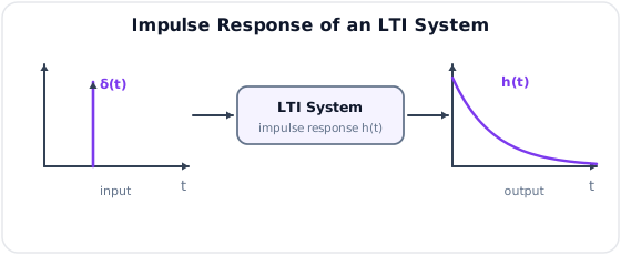
Why the Impulse Is Used as a Test Signal
The impulse is the natural probe for an LTI system because any signal can be built from scaled, shifted impulses. Using the sifting property, a discrete input is written as
and a continuous input as
Now apply the two LTI properties:
- Time-invariance — the response to a shifted impulse \(\delta[n-k]\) is the shifted impulse response \(h[n-k]\).
- Linearity — the response to a weighted sum of impulses is the same weighted sum of the individual responses.
So the output is that same combination of shifted impulse responses:
which is exactly convolution (next section). This is why \(h(t)\) or \(h[n]\) alone is a complete "fingerprint" of an LTI system: know it, and you know the response to every input.
System Properties from the Impulse Response
Likely Exam Question (5–10 marks)
"How can the causality, stability, and memory of an LTI system be judged from its impulse response?"
For an LTI system, each system property reduces to a simple condition on \(h(t)\) / \(h[n]\):
| Property | Continuous-time condition | Discrete-time condition | Meaning |
|---|---|---|---|
| Memoryless | \(h(t)=K\delta(t)\) | \(h[n]=K\delta[n]\) | Output depends only on the present input |
| Causal | \(h(t)=0\) for \(t<0\) | \(h[n]=0\) for \(n<0\) | No output before the input is applied |
| BIBO stable | \(\int_{-\infty}^{\infty}\lvert h(t)\rvert\,dt<\infty\) | \(\sum_{n=-\infty}^{\infty}\lvert h[n]\rvert<\infty\) | Bounded input always gives bounded output |
| Invertible | \(\exists\,h_{\text{inv}}\) with \(h*h_{\text{inv}}=\delta(t)\) | \(\exists\,h_{\text{inv}}\) with \(h*h_{\text{inv}}=\delta[n]\) | Input can be recovered from output |
These tests follow directly from convolution:
- Memoryless: if \(h(t)=K\delta(t)\), then \(y(t)=x(t)*K\delta(t)=Kx(t)\), so the output uses only the present input. Any delayed or spread component in \(h(t)\) introduces memory.
- Causal: in \(y(t)=\int x(\tau)h(t-\tau)d\tau\), a causal system must not use values with \(\tau>t\). This is guaranteed precisely when \(h(t-\tau)=0\) for \(t-\tau<0\), or \(h(v)=0\) for \(v<0\).
- Stable: if \(\lvert x(t)\rvert\leq M\), use the convolution bound
Therefore, absolute integrability of \(h(t)\) guarantees a bounded output. The discrete proof replaces the integral by a sum.
- Invertible: cascading the system with its inverse must produce the identity system, whose impulse response is \(\delta\); hence \(h*h_{\text{inv}}=\delta\).
BIBO stability is the most-asked: an LTI system is stable if and only if its impulse response is absolutely integrable (continuous) or absolutely summable (discrete).
Example. Is \(h(t)=e^{-2t}u(t)\) causal and stable?
- Causal: \(h(t)=0\) for \(t<0\) because of \(u(t)\) ✓
- Stable: \(\displaystyle\int_{0}^{\infty} e^{-2t}\,dt = \tfrac{1}{2} < \infty\) ✓ — absolutely integrable, so BIBO stable.
Contrasting examples: \(h(t)=u(t)\) is causal but unstable because its absolute integral is infinite. In contrast, \(h(t)=e^tu(-t)\) is stable because \(\int_{-\infty}^{0}e^t dt=1\), but it is noncausal because it is nonzero for \(t<0\).
Step Response and Impulse Response
The step response \(s(t)\) is the output for a unit-step input \(u(t)\). Since the unit step is the running integral of the impulse, the step and impulse responses form an integral–derivative pair:
Discrete-time (accumulation and first difference):
This lets you obtain either response from the other — a common short-question twist.
Impulse Response and Transfer Function
Transforming the impulse response gives the system's transfer/frequency characterisation:
So \(H(s)\) is the Laplace transform and \(H(\omega)\) the Fourier transform of \(h(t)\), and convolution in time becomes multiplication in these domains: \(y=x*h \Leftrightarrow Y=XH\).
Complex exponentials are the eigenfunctions of LTI systems:
the system merely scales them by \(H(s)\). Finally, the duration of the impulse response classifies digital filters:
| Impulse response | Filter type |
|---|---|
| Finite duration (finitely many nonzero terms) | FIR |
| Infinite duration | IIR |
(treated in detail in the System Equations & Digital Filters chapter).
3. Convolution
Likely Exam Question (10 marks)
"Explain convolution and state its use in finding the response of an LTI system."
Definition
Convolution is the mathematical operation that combines an input signal with the impulse response of an LTI system to determine its output. It accounts for the response produced by every past input value and adds all those contributions at the observation time.
For continuous-time signals:
For discrete-time signals:
Why an LTI System Produces Convolution
Any continuous-time input can be decomposed into a continuum of shifted impulses:
Here, \(x(\tau)\delta(t-\tau)\,d\tau\) is an impulse at \(t=\tau\) whose infinitesimal weight is \(x(\tau)d\tau\). If the response of the system to \(\delta(t)\) is \(h(t)\), time invariance makes the response to \(\delta(t-\tau)\) equal to \(h(t-\tau)\). By linearity, each response is multiplied by \(x(\tau)d\tau\), and all responses may be added. Therefore,
The same argument for a discrete sequence,
gives
Hence convolution is not merely a calculation rule: it follows directly from the linearity and time invariance of the system.
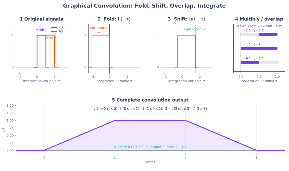
Graphical Convolution Steps
For graphical continuous-time convolution, keep \(x(\tau)\) fixed and operate on \(h(\tau)\):
- Fold: reflect \(h(\tau)\) about the vertical axis to obtain \(h(-\tau)\).
- Shift: move the folded signal by \(t\) to obtain \(h(t-\tau)\).
- Multiply: form the point-by-point product \(x(\tau)h(t-\tau)\).
- Integrate: the signed area of the product gives one output value \(y(t)\).
- Slide and repeat: vary \(t\) from \(-\infty\) to \(+\infty\) to obtain the complete output waveform.
Thus the value of \(y(t)\) is large where the two signals have a large overlap and is zero where they do not overlap.
Properties of Convolution
Convolution (\(*\)) combines two signals to form a third and is the foundation of Linear Time-Invariant (LTI) system analysis. The following properties simplify interconnected LTI systems and are frequently asked directly in examinations.
Core Algebraic Properties
1. Commutative Property
Starting with the definition and substituting \(\lambda=t-\tau\),
which is \(h*x\). Therefore, the order of the two signals does not affect the convolution result.
2. Associative Property
The grouping of successive convolutions can be changed without changing the output. Physically, if two LTI systems with impulse responses \(h\) and \(g\) are connected in cascade, their overall impulse response is \(h*g\), regardless of which pair is convolved first. This permits a complicated cascade to be replaced by one equivalent system.
3. Distributive Property
This follows by distributing the integral over addition:
It represents two LTI systems connected in parallel: the total output equals the sum of the individual outputs.
Operational Properties
4. Identity and Impulse-Shift Property
The unit impulse is the identity element of convolution:
Using the sifting property,
Thus convolution with an impulse reproduces the signal, while convolution with a shifted impulse reproduces and shifts it.
5. Time-Shift Property
If \(y(t)=x(t)*h(t)\), then shifting either input shifts the output by the same amount, and shifting both inputs shifts the output by the sum of the delays:
The single-shift case \(x(t-t_0)*h(t)=x(t)*h(t-t_0)=y(t-t_0)\) is the convolution form of time invariance.
6. Time-Scaling Property
Compressing or expanding the time axis of both inputs by the same factor \(a\) scales the output in time and scales its amplitude by \(1/|a|\):
7. Differentiation Property
Differentiation may be applied to either member of a convolution:
This is useful when differential equations or step and impulse responses are involved.
8. Area and Duration Properties
For absolutely integrable signals, the area under a convolution is the product of the individual areas:
If two finite-duration signals occupy intervals of lengths \(T_x\) and \(T_h\), their convolution generally has duration \(T_x+T_h\) (endpoint conventions aside). The output begins when the signals first overlap and ends when their overlap disappears.
Transform-Domain Property
9. Convolution Theorem
Convolution in the time domain is equivalent to point-wise multiplication in the frequency domain, which turns a difficult integral into a simple product via the Fourier or Laplace transform:
The Laplace-domain form \(\mathcal{L}\{x(t)*h(t)\}=X(s)\,H(s)\) is the basis of transfer-function analysis: the output transform is the input transform multiplied by the system transfer function.
Solved Example - Discrete Convolution
Q. Find \(y[n]=x[n]*h[n]\) when \(x[0]=1\), \(x[1]=2\) and \(h[0]=1\), \(h[1]=1\); all other samples are zero.
For two length-2 sequences, the linear-convolution length is \(2+2-1=3\). Using
the three non-zero output samples are:
Therefore,
![Discrete convolution example: x[n]={1,2} convolved with h[n]={1,1} gives y[n]={1,3,2}, shown as stem plots](.././img/conv_example_stem.svg)
Key Exam Points - LTI Systems and Convolution
- LTI = linearity + time invariance; fully described by its impulse response \(h\).
- Output of an LTI system is convolution of input with impulse response: \(y=x*h\).
- Causal: \(h(t)=0\) for \(t<0\). BIBO stable: \(h\) absolutely integrable/summable.
- Convolution: fold → shift → multiply → integrate; commutative, associative, distributive.
- Convolution in time ↔ multiplication in frequency (\(X(\omega)H(\omega)\)).
Model Answer — LTI System and Its Properties [5 marks]
Exam-ready answer
Let a system be the operator \(T\{\cdot\}\) with input \(x\) and output \(y=T\{x\}\). It is linear when it obeys superposition for arbitrary inputs and constants:
This combines additivity and homogeneity. It is time invariant when a delay at the input creates exactly the same delay at the output:
A system satisfying both tests is LTI. Its response is completely determined by the impulse response \(h=T\{\delta\}\):
| Property | CT impulse-response test | DT test |
|---|---|---|
| Causal | \(h(t)=0\) for \(t<0\) | \(h[n]=0\) for \(n<0\) |
| BIBO stable | \(\int_{-\infty}^{\infty}\lvert h(t)\rvert dt<\infty\) | \(\sum_{n=-\infty}^{\infty}\lvert h[n]\rvert<\infty\) |
| Memoryless | \(h(t)=K\delta(t)\) | \(h[n]=K\delta[n]\) |
The stability test follows directly: if \(|x(t)|\le M\), then
which is finite when \(h\) is absolutely integrable. For example, \(h(t)=e^{-2t}u(t)\) is causal and stable because it vanishes for \(t<0\) and \(\int_0^\infty e^{-2t}dt=1/2\). By contrast, \(h(t)=u(t)\) is causal but unstable because its absolute integral diverges. These tests assume an LTI system; for a nonlinear or time-varying system, \(h\) alone does not characterize every input response.
Practice target: 9 minutes; state both operator tests, the convolution relation, and prove the BIBO bound before classifying one example.
Model Answer — Impulse Response and Convolution Derivation [5 marks]
Exam-ready answer
The impulse response \(h(t)\) of a CT system is its zero-state output to the unit impulse: \(h(t)=T\{\delta(t)\}\). For a DT system, \(h[n]=T\{\delta[n]\}\). In an LTI system it is a complete description because every input is a weighted superposition of shifted impulses.
By the sifting identity, write a CT input as
Now apply the two assumptions step by step. Time invariance makes the response to \(\delta(t-\tau)\) equal to \(h(t-\tau)\). Linearity multiplies that response by \(x(\tau)d\tau\) and permits all component responses to be added. Hence
Similarly,
As a quick example, if \(h[n]=\delta[n]+\tfrac12\delta[n-1]\), the shift property gives \(y[n]=x[n]+\tfrac12x[n-1]\): the present sample and one delayed sample are weighted and added. Transforming the convolution yields \(Y=XH\), so the Fourier, Laplace or z-transform of \(h\) is the system frequency response or transfer function. Thus impulse testing is useful precisely because LTI superposition converts one measured response into the response for every admissible input.
Practice target: 8 minutes; begin with the impulse decomposition and label where time invariance and linearity are used in the three-line derivation.
Model Answer — Convolution and LTI-System Response [10 marks]
Exam-ready answer
Convolution combines an input with an LTI system’s impulse response to sum the contribution of every shifted input component at the observation time. Its CT and DT definitions are
Here \(\tau\) or \(k\) is a dummy integration/summation variable, and \(t\) or \(n\) is the output time. The formula follows by decomposing \(x(t)=\int x(\tau)\delta(t-\tau)d\tau\): time invariance changes each shifted impulse into \(h(t-\tau)\) and linearity sums the weighted responses.
For graphical CT convolution, keep \(x(\tau)\) fixed and perform:
- Fold \(h(\tau)\) about the origin to obtain \(h(-\tau)\).
- Shift by the observation time to form \(h(t-\tau)\).
- Multiply point by point with \(x(\tau)\).
- Integrate the signed product area to get one value \(y(t)\).
- Slide through all \(t\) to trace the complete output.
For two unit-height rectangular pulses supported on \(0\le t\le1\), the overlap length is the output. Therefore
a triangular waveform. This explicitly shows that finite supports of lengths \(T_x\) and \(T_h\) produce support length \(T_x+T_h\) between first and last overlap (with endpoint conventions not affecting duration).
DT worked example: let \(x[n]=\{1,2\}\) and \(h[n]=\{1,1\}\), both beginning at \(n=0\). The output length is \(2+2-1=3\):
Important checks are \(x*h=h*x\), \(x*\delta=x\), and \(\mathcal F\{x*h\}=X(\omega)H(\omega)\). For causal signals, the effective limits reduce to past values only; for example \(y(t)=\int_0^t x(\tau)h(t-\tau)d\tau\) when both causal. Consequently convolution predicts transient and steady response, combines cascaded LTI systems, and converts to multiplication in a transform domain for efficient calculation.
Practice target: 18 minutes; write both definitions, draw all four graphical operations, derive the rectangular-pulse regions and verify one discrete sequence.
Model Answer — Properties of Convolution [2–5 marks]
Exam-ready answer
For \(y(t)=x(t)*h(t)=\int_{-\infty}^{\infty}x(\tau)h(t-\tau)d\tau\), the principal properties are:
| Property | Formula | System meaning |
|---|---|---|
| Commutative | \(x*h=h*x\) | input and impulse response may be interchanged mathematically |
| Associative | \((x*h_1)*h_2=x*(h_1*h_2)\) | cascaded LTI systems may be grouped freely |
| Distributive | \(x*(h_1+h_2)=x*h_1+x*h_2\) | parallel branch outputs add |
| Identity | \(x*\delta=x\) | impulse is the convolution identity |
| Shift | \(x*\delta(t-t_0)=x(t-t_0)\) | a shifted impulse delays the signal |
Commutativity follows by substituting \(v=t-\tau\) in the definition. Distributivity follows from splitting the integral over a sum. A shift is proved by sifting:
Other useful results are
and, for absolutely integrable signals,
The convolution theorem states
with corresponding Laplace and z-transform forms. Thus time-domain convolution can be evaluated as transform-domain multiplication. For a 2-mark response, state commutative, associative, distributive and identity properties; for 5 marks, add shift, differentiation, the convolution theorem and one brief proof.
Practice target: 6 minutes for the complete 5-mark response; do not confuse convolution in time with multiplication in time, which produces scaled convolution in frequency.