Information Theory and Signal Transmission
Possible Exam Questions
Exam Questions and Answer Map
Evidence note: [PYQ paper/year] = exact question observed in that past paper; [likely] = pattern-predicted variant not confirmed as exact PYQ.
-
Define information, entropy and channel capacity; state the Shannon-Hartley law. [5–10] — [likely]
-
Answer plan: Define information \(I=-\log_2 P\) → define entropy \(H=-\sum p_i\log_2 p_i\) → state Nyquist capacity \(C=2B\log_2 M\) → state Shannon-Hartley \(C=B\log_2(1+S/N)\) → interpret each variable.
-
Model answer: Information, Entropy and Channel Capacity
-
Explain the effect of signal-to-noise ratio and bandwidth on channel capacity. [5] — [likely]
-
Answer plan: Write Shannon formula → show C increases with B but with diminishing returns → show C increases logarithmically with SNR → discuss bandwidth–SNR trade-off → cite practical implication (e.g. spread spectrum trades BW for noise tolerance).
-
Model answer: Bandwidth, SNR and Channel Capacity
-
Explain baseband and passband signal transmission; state what limits reliable transmission. [5] — [likely]
-
Answer plan: Define baseband (no carrier) vs passband (message modulated onto a carrier) → give spectral location and typical media → list impairments (attenuation, noise, bandwidth limitation, distortion, interference) → state distortionless condition (\(\lvert H(\omega)\rvert=K\), linear phase).
- Model answer: Baseband and Passband Transmission
1. Information Theory
Likely Exam Question (5 marks)
"State Shannon-Hartley theorem. Define information, entropy, and channel capacity."
Information Content
Information theory measures the amount of uncertainty removed when a message is received. If an event has probability \(P\), its information content is:
Less probable events carry more information.
Entropy
For a source with symbols \(x_i\) and probabilities \(p_i\), average information per symbol is called entropy:
Entropy is maximum when all symbols are equally likely. It represents the minimum average number of bits needed to encode a source symbol without loss.
Channel Capacity
Channel capacity is the maximum reliable information rate that can be transmitted over a channel.
For a noiseless channel with bandwidth \(B\) and \(M\) signaling levels:
For a noisy band-limited channel, Shannon-Hartley theorem gives:
where:
- \(B\) = channel bandwidth in Hz
- \(S/N\) = signal-to-noise power ratio
- \(C\) = maximum error-free data rate in bps
Derivation of the Noiseless (Nyquist) Capacity
A channel band-limited to \(B\) Hz cannot carry pulses at an unlimited rate. By the Nyquist signaling criterion, the largest symbol (pulse) rate that a channel of bandwidth \(B\) can carry without inter-symbol interference is
This is the dual of the sampling theorem: a signal strictly band-limited to \(B\) Hz is fully described by \(2B\) samples per second, so at most \(2B\) independent pulses per second can be sent and still be resolved at the receiver.
If each pulse is allowed to take one of \(M\) equally likely, distinguishable amplitude levels, then each symbol carries
because \(M\) levels encode \(\log_2 M\) bits. The capacity is the symbol rate multiplied by the information per symbol:
In a truly noiseless channel there is no bound on \(M\) — levels can be packed arbitrarily close — so \(C\) could be made infinite. Noise destroys this freedom, which leads directly to the Shannon-Hartley limit.
Exam-Oriented Derivation of the Noisy (Shannon-Hartley) Capacity
The following is an exam-oriented proof sketch built from differential entropy and mutual information. A fully rigorous proof additionally treats the band-limited Gaussian channel as a set of independent orthogonal modes and invokes the channel-coding theorem.
Step 1 - Channel Model and Mutual Information
The channel adds independent noise \(N\) to the transmitted signal \(X\) to form the received signal \(Y\):
The information delivered per sample is the mutual information \(I(X;Y)\) — the amount by which knowing \(X\) reduces the uncertainty of \(Y\):
Because \(Y = X + N\), once \(X\) is perfectly known the only remaining uncertainty in \(Y\) comes from the noise. Hence \(H(Y\mid X) = H(N)\), giving
where \(H(\cdot)\) denotes differential entropy.
Step 2 - Maximum Entropy of the Noise and Output
For a fixed average power (variance), the Gaussian distribution maximizes differential entropy. Two facts follow.
- Noise — assuming additive white Gaussian noise (AWGN) of power \(N\):
- Output — the signal power is \(S\) and the noise power is \(N\). As signal and noise are independent, the output power is \(S + N\). Entropy \(H(Y)\) is largest when \(Y\) is also Gaussian (which requires the input \(X\) to be Gaussian):
Step 3 - Capacity per Sample
Subtracting the noise entropy from the maximum output entropy gives the greatest information carried by one independent sample:
Using \(\log A - \log B = \log(A/B)\), the common factor \(2\pi e\) cancels:
Step 4 - Scaling to Continuous Time
By the Nyquist sampling theorem, a channel of bandwidth \(B\) Hz provides exactly \(2B\) independent samples per second. Multiplying the per-sample capacity by this sampling rate gives the continuous-channel capacity:
The factors of \(2\) cancel, producing the classic Shannon-Hartley theorem:
This is the supremum of reliable data rates over a band-limited channel corrupted by AWGN. For every rate \(R<C\), sufficiently long and suitable coding can make the probability of error arbitrarily small; rates above \(C\) cannot be made reliable. It does not promise literally zero error with a finite code.
Important Points
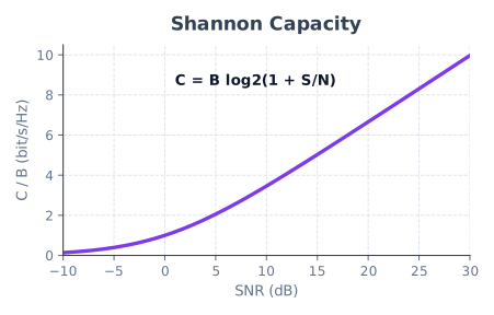
- At a fixed numerical value of \(S/N\), increasing bandwidth increases capacity linearly.
- Increasing \(S/N\) increases capacity logarithmically.
- Capacity gives a theoretical limit; practical systems approach it using efficient modulation and coding.
If signal power \(S\) and white-noise spectral density \(N_0\) are fixed, total noise power grows with bandwidth, \(N=N_0B\), and
so capacity still increases with \(B\), but not linearly and with diminishing returns.
Solved Example - Shannon-Hartley Capacity
Q. A channel has bandwidth \(B = 3\,\text{kHz}\) and \(S/N = 30\,\text{dB}\). Find its capacity.
Convert dB to linear ratio:
2. Transmission of Signals
Likely Exam Question (5 marks)
"Explain baseband and passband signal transmission. What factors limit reliable transmission?"
Signal Transmission
Signal transmission is the process of carrying information from a source to a destination through a physical medium such as copper cable, optical fiber, or free space.
Basic communication chain:

Baseband Transmission
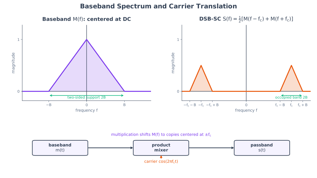
In baseband transmission, the information-bearing waveform is sent directly without translating it to a high-frequency carrier. Its spectrum remains centered around zero frequency (DC). For digital data, the bit sequence is converted into a line-coded pulse waveform such as NRZ or Manchester coding and applied directly to a low-pass channel.
Baseband transmission is appropriate when the medium can pass frequencies down to or near DC. The transmitter mainly performs pulse shaping or line coding, while the receiver uses filtering, equalization, timing recovery, and regeneration. It is simple and efficient over dedicated wired links, but it cannot directly share a radio-frequency channel by carrier allocation.
Examples:
- Digital data over short wired links
- Ethernet baseband signaling
- PCM pulses before modulation
Passband Transmission
In passband transmission, the message modifies a parameter of a sinusoidal carrier and shifts its spectrum from baseband to a band centered around the carrier frequency \(f_c\). A general modulated waveform may be written as
where the message controls amplitude \(A(t)\), phase \(\phi(t)\), or instantaneous frequency. For example, multiplying a message by a carrier gives \(s(t)=m(t)\cos\omega_ct\) and produces translated spectral components around \(\pm\omega_c\).
Modulation is required for practical antenna size, efficient radiation, frequency-division multiplexing, spectrum allocation, and transmission through band-pass media. The transmitter therefore contains a modulator and RF stages, while the receiver must select the desired channel and demodulate it back to baseband.
Examples:
- AM, FM, PM radio
- Mobile communication
- Satellite communication
| Feature | Baseband Transmission | Passband Transmission |
|---|---|---|
| Spectral location | Centered near \(0\) Hz | Centered near carrier \(f_c\) |
| Carrier modulation | Not required | Required |
| Typical medium | Wired low-pass channel | Radio, satellite, band-pass cable channel |
| Main transmitter operation | Line coding and pulse shaping | Modulation and frequency translation |
| Receiver operation | Equalization and pulse detection | RF selection, demodulation, then baseband recovery |
Factors Affecting Transmission
| Factor | Effect |
|---|---|
| Bandwidth limitation | Causes waveform spreading and inter-symbol interference |
| Noise | Random disturbance that reduces \(S/N\) |
| Attenuation | Signal power decreases with distance |
| Distortion | Different frequency components are altered unequally |
| Interference | Unwanted signals from other sources |
Distortionless Transmission
A system gives distortionless transmission if the output is only a scaled and delayed version of the input:
In frequency domain, this requires:
- Constant magnitude response: \(\lvert H(\omega)\rvert = K\)
- Linear phase response: \(\angle H(\omega) = -\omega t_d\)
These conditions need to hold over the occupied frequency band of the input signal, not necessarily over all frequencies. Constant magnitude prevents amplitude distortion, while linear phase gives every spectral component the same time delay and therefore prevents phase distortion.
Key Exam Points - Information Theory & Transmission
- Information content: \(I = -\log_2 P\) bits; entropy \(H = -\sum p_i\log_2 p_i\) bits/symbol.
- Noiseless (Nyquist) capacity: \(C = 2B\log_2 M\); noisy (Shannon-Hartley): \(C = B\log_2(1+S/N)\).
- Bandwidth raises capacity linearly; SNR raises it only logarithmically (use linear \(S/N\), not dB).
- Baseband = no carrier (low-pass channel); passband = message modulated onto a carrier.
- Distortionless transmission: constant \(\lvert H(\omega)\rvert\) and linear phase over the signal band.
Model Answer — Information, Entropy and Channel Capacity [5–10 marks]
5-mark answer and 10-mark extension
For 5 marks — write this
The self-information obtained when an event of probability \(p_i\) occurs is
Thus a rare event conveys more information, independent events add information, and an event certain to occur conveys zero information. The entropy of a discrete source is its average information per symbol:
\(H\) is nonnegative and is maximum at \(\log_2M\) for \(M\) equiprobable symbols. Channel capacity \(C\) is the supremum of rates at which information can be transmitted with arbitrarily small error using suitable coding.
For a noiseless band-limited channel and \(M\) distinguishable levels, Nyquist gives
For an AWGN channel of bandwidth \(B\) Hz, signal power \(S\) and in-band noise power \(N\),
is the Shannon–Hartley law. The ratio \(S/N\) must be linear, not in decibels.
Add for a 10-mark variant
Nyquist follows because a channel of bandwidth \(B\) supports at most \(2B\) independent symbols per second, and each of \(M\) levels carries \(\log_2M\) bits. Shannon’s noisy result can be motivated from the real AWGN sample model \(Y=X+Z\). The mutual information per independent sample is
For fixed variance, a Gaussian variable has maximum differential entropy. With independent powers \(S\) and \(N\),
so the maximum information is \(\tfrac12\log_2(1+S/N)\) bit per real sample. A \(B\)-Hz channel has \(2B\) real degrees of freedom per second; multiplication gives \(C=B\log_2(1+S/N)\). The assumptions are an ideal band-limited channel, additive white Gaussian noise, average input-power constraint, and coding over sufficiently long blocks. Rates \(R<C\) can approach arbitrarily small error probability; Shannon does not promise zero error for finite codes.
Worked examples. A binary equiprobable source has
For \(B=3\,\text{kHz}\) and \(S/N=30\,\text{dB}\), first convert \(S/N=10^{30/10}=1000\):
Entropy measures source uncertainty; capacity measures the channel’s reliable-rate limit. Source coding tries to approach \(H\), whereas channel coding permits reliable operation below \(C\).
Practice target: 9 minutes for the 5-mark core or 18 minutes for the derivation and examples; define every symbol and convert dB before substitution.
Model Answer — Bandwidth, SNR and Channel Capacity [5 marks]
Exam-ready answer
For a channel corrupted by additive white Gaussian noise, the Shannon–Hartley limit is
where \(B\) is bandwidth in hertz, \(S\) is received signal power and \(N\) is noise power measured in the same bandwidth. Reliable coded transmission is theoretically possible for \(R<C\) and impossible for \(R>C\).
| Change | Capacity effect | Engineering interpretation |
|---|---|---|
| Increase \(S/N\) at fixed \(B\) | Logarithmic increase | Each doubling of \(1+S/N\) adds only \(B\) bit/s |
| Increase \(B\) while keeping numerical \(S/N\) fixed | Linear increase | More independent signal dimensions are available |
| Increase \(B\) with fixed \(S\) and white-noise density \(N_0\) | Increasing, but with diminishing return | Noise grows as \(N=N_0B\) |
In the physically important fixed-\(S\), fixed-\(N_0\) case,
Increasing \(B\) lowers the received SNR per degree of freedom, so capacity approaches the finite wideband limit \(S/(N_0\ln2)\) rather than growing without bound. Conversely, at fixed bandwidth, large power increases produce progressively smaller gains because of the logarithm.
Numerical comparison: with \(B=1\,\text{MHz}\) and \(S/N=15\,\text{dB}\), the linear ratio is \(10^{1.5}=31.62\), hence
Doubling the SNR to \(63.24\) gives only \(C\approx6.01\) Mbit/s, about 0.98 Mbit/s more. Practical systems therefore trade bandwidth, transmit power, coding gain and modulation order: spread-spectrum or low-rate coded links spend extra bandwidth to operate reliably at low SNR, while spectrum-limited links demand higher SNR and efficient modulation.
Practice target: 8 minutes; state both the fixed-SNR and fixed-noise-density cases and show one dB-to-linear calculation.
Model Answer — Baseband and Passband Transmission [5 marks]
Exam-ready answer
Baseband transmission sends the information waveform without translating it to a carrier; its spectrum is centred at zero frequency. A low-pass medium that passes DC or near-DC is required. Line coding, pulse shaping, equalisation and regeneration are typical operations, as in an Ethernet wired link.
Passband transmission modulates the message onto a carrier \(f_c\), placing the spectrum around \(\pm f_c\). For example,
| Feature | Baseband | Passband |
|---|---|---|
| Spectral centre | \(0\) Hz | carrier \(f_c\) |
| Carrier/modulator | Not required | Required |
| Typical channel | low-pass cable | radio, satellite or band-pass cable |
| Examples | line-coded data, PCM pulses | AM, FM, PSK, QAM |
Passband operation enables practical antennas, spectrum allocation, frequency-division multiplexing and transmission through a band-pass channel. In either case the complete path is source → transmitter → channel → receiver → destination.
Reliable transmission is limited by attenuation, finite bandwidth, additive noise, interference, fading and amplitude/phase distortion. For an LTI channel to be distortionless over the occupied input band, its output must be only scaled and delayed:
Therefore \(|H(\omega)|=K\) must be constant and \(\angle H(\omega)=-\omega t_d\) linear over that band. Constant magnitude prevents unequal attenuation; linear phase gives every spectral component the same group delay. Equalisers compensate channel distortion, filters reject out-of-band noise, and coding detects or corrects residual errors.
Practice target: 9 minutes; draw both spectral locations, give one example of each mode, list the five impairments and finish with the distortionless condition.