PCM and ADPCM
Possible Exam Questions
Exam Questions and Answer Map
Evidence note: [PYQ paper/year] = exact question observed in that past paper; [likely] = pattern-predicted variant not confirmed as an exact PYQ.
- Draw the generic block diagram of a PCM transmitter and receiver and explain each component in brief. [5+5=10] — [PYQ 2079]
- Answer plan: Transmitter [5]: anti-alias LPF -> sampler/S&H -> quantizer -> encoder -> line coder; Receiver [5]: regenerative receiver -> line decoder -> code decoder/DAC -> reconstruction LPF -> destination; state the role of synchronization.
-
Model answer: PCM Transmitter and Receiver
-
Explain PCM and state its advantages in digital communication. [5] — [likely; PCM was a 3-mark limb in NTC 2081]
- Answer plan: Define PCM -> list sampling, quantization and encoding -> explain 3R regeneration, TDM compatibility, encryption, switching and stable quality -> state quantization noise and bandwidth cost.
-
Model answer: PCM Principle and Advantages
-
A speech channel is sampled at \(8\,\text{kHz}\) and encoded with 8 bits/sample. Find the bit rate, ideal minimum binary baseband bandwidth and SQNR. [5] — [likely]
- Answer plan: \(R_b=nf_s=64\,\text{kbps}\) -> ideal Nyquist \(B_{min}=R_b/2=32\,\text{kHz}\) for two-level signaling -> \(SQNR\approx6.02(8)+1.76=49.92\,\text{dB}\) for a full-scale sine -> qualify practical bandwidth and companding.
-
Model answer: PCM Rate, Bandwidth and SQNR Example
-
Differentiate PCM, DPCM and ADPCM. Why can ADPCM transmit speech at a lower bit rate? [10] — [likely]
- Answer plan: PCM sends absolute sample -> DPCM sends prediction error -> ADPCM adapts predictor and quantizer -> compare bits/sample, rate, complexity, quality and applications -> explain adjacent-sample correlation and smaller error variance.
-
Model answer: PCM, DPCM and ADPCM Comparison
-
Explain delta modulation. What are slope-overload distortion and granular noise, and how does adaptive delta modulation reduce them? [10] — [likely]
- Answer plan: Define one-bit DPCM staircase -> describe comparator/integrator loop -> derive tracking-slope condition -> explain small-step slope overload and large-step granular noise -> show adaptive step-size remedy.
-
Model answer: Delta Modulation and Tracking Errors
-
Compare PCM and ADPCM with respect to principle, bit rate, bandwidth, complexity, noise and applications. [5] — [likely]
- Answer plan: Use a two-column table -> PCM absolute 8-bit sample and 64 kbps -> ADPCM adaptive prediction error, commonly 4-bit and 32 kbps -> discuss state dependence, error propagation and speech applications.
- Model answer: PCM versus ADPCM
1. Digital Speech-Coding Context
An analog speech waveform is continuous in time and amplitude. A waveform coder converts it to digital form while preserving enough sample information for acceptable reconstruction.
The basic families are:
- PCM: encode the absolute quantized sample.
- DPCM: predict the sample and encode only the prediction error.
- ADPCM: adapt the predictor and/or quantizer to changing speech statistics.
- Delta modulation: one-bit differential coding with an oversampled staircase.
Sampling, quantization and companding fundamentals are developed in 5.4 Analog-to-Digital Conversion.
2. Pulse Code Modulation (PCM)
Pulse Code Modulation represents each analog sample by a binary codeword. Its three defining operations are:
- Sampling: take values at intervals \(T_s\).
- Quantization: round each value to one of \(L=2^n\) levels.
- Encoding: represent the selected level by an \(n\)-bit word.
PCM is digital even though its source may be analog. PAM alone is not digital because PAM pulse amplitudes remain continuous.
PCM Transmitter
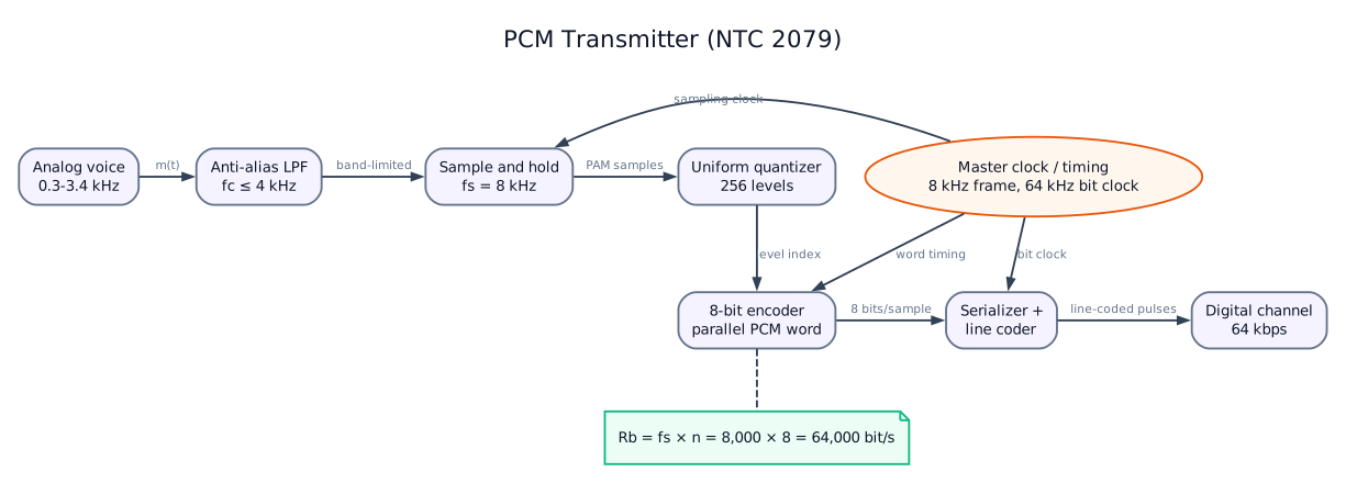
| Block | Function |
|---|---|
| Anti-aliasing LPF | Limit the message to \(f_m<f_s/2\) |
| Sampler / S&H | Produce stable samples at \(f_s\) |
| Compressor, when used | Reduce dynamic range before uniform quantization |
| Quantizer | Select one of \(2^n\) amplitude levels |
| Encoder | Convert level index to an \(n\)-bit codeword |
| Parallel/serial and line coder | Form the serial channel waveform and support clock recovery |
The encoder output is a sequence of codewords, not a direct copy of the analog waveform.
PCM Receiver
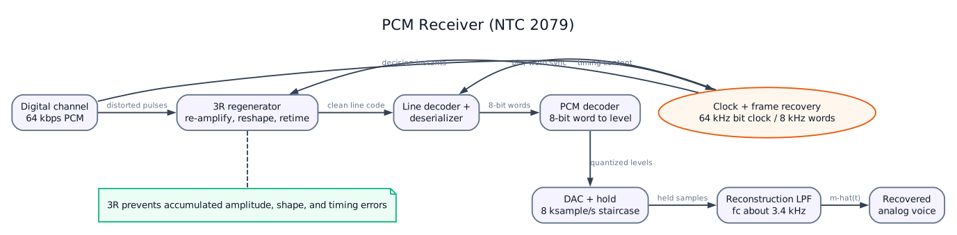
| Block | Function |
|---|---|
| Input filter/equalizer | Limit noise and compensate channel distortion |
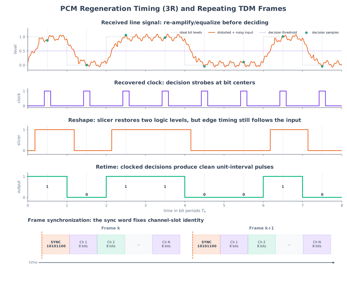
| Clock recovery and regenerator | Retiming, reshaping and re-amplification of bits |
| Line decoder / de-framer | Recover binary codewords and channel positions |
| Decoder and DAC | Map each codeword to its quantized sample level |
| Expander, when used | Invert transmitter compression |
| Reconstruction LPF | Suppress sample images and smooth the staircase |
The reconstructed output differs from the original by quantization error and any bit errors or filtering distortion.
PCM Bit Rate and Bandwidth
For \(n\) bits/sample at sampling frequency \(f_s\):
For \(N\) time-division-multiplexed channels, ignoring framing/signaling overhead:
For ideal binary baseband transmission with zero intersymbol interference, the Nyquist lower bound is:
This is a theoretical lower bound for two-level signaling. Actual occupied bandwidth depends on line code, pulse shaping, roll-off and channel constraints. Manchester, for example, needs more bandwidth than suitably pulse-shaped NRZ.
Standard Telephone PCM
| Quantity | Value |
|---|---|
| Speech passband | Approximately \(300\) to \(3400\,\text{Hz}\) |
| Sampling rate | \(8\,\text{kHz}\) |
| Sampling period | \(125\,\mu\text{s}\) |
| Codeword length | 8 bits/sample |
| Channel bit rate | \(64\,\text{kbps}\) |
Ideal two-level Nyquist bandwidth:
Ideal full-scale-sine quantization SQNR:
Telephone companding changes SQNR versus input level, so the last value is not a universal speech-channel SQNR.
PCM Advantages
- Regenerative repeaters prevent progressive analog noise accumulation.
- Stable quality over long digital links.
- Natural compatibility with TDM and digital switching.
- Easy encryption, storage, processing and error control.
- A common digital network can carry voice, data and signaling.
- IC implementation gives repeatable characteristics.
PCM Limitations
- Usually greater bandwidth than the original analog message.
- Quantization noise is unavoidable at finite resolution.
- Requires accurate sampling and bit/frame synchronization.
- Converter and timing circuitry add complexity and power.
- A bit error may cause a large sample error, especially in a significant bit.
3. Quantization Noise, Companding and Bit Errors
Quantization Noise
For an ideal uniform quantizer with step \(\Delta\):
For a full-scale sinusoid:
Each additional bit improves ideal SQNR by about \(6\,\text{dB}\), but also increases channel bit rate by \(f_s\) bits/s.
Companded PCM
Speech has a large dynamic range and spends substantial time near zero. A-law or \(\mu\)-law compression before quantization allocates relatively finer resolution to weak speech. The receiver expands the decoded values.
Companding improves low-level speech performance but may increase distortion for large signals compared with a uniform quantizer of the same nominal step near full scale.
Transmission Error Effect
Natural-binary PCM codewords are sensitive to bit significance: an MSB error changes the sample far more than an LSB error. Gray coding can make adjacent quantizer levels differ by one bit, but conventional telephony PCM uses standardized code assignments and relies on a sufficiently low channel BER.
4. PCM Framing and Synchronization
In a multiplexed PCM system, the receiver must identify:
- Individual bit boundaries.
- The \(n\) bits belonging to one sample word.
- Frame boundaries.
- The time slot assigned to each channel.
Framing patterns or dedicated framing slots allow alignment. Loss of frame alignment can route sample words to the wrong channels even when individual bits are received correctly.
Line coding such as HDB3 maintains physical-layer timing transitions; framing identifies the logical TDM structure. These are different functions.
5. Differential PCM (DPCM)
Adjacent speech samples are strongly correlated. DPCM predicts the current sample from previous reconstructed samples and transmits only the difference.
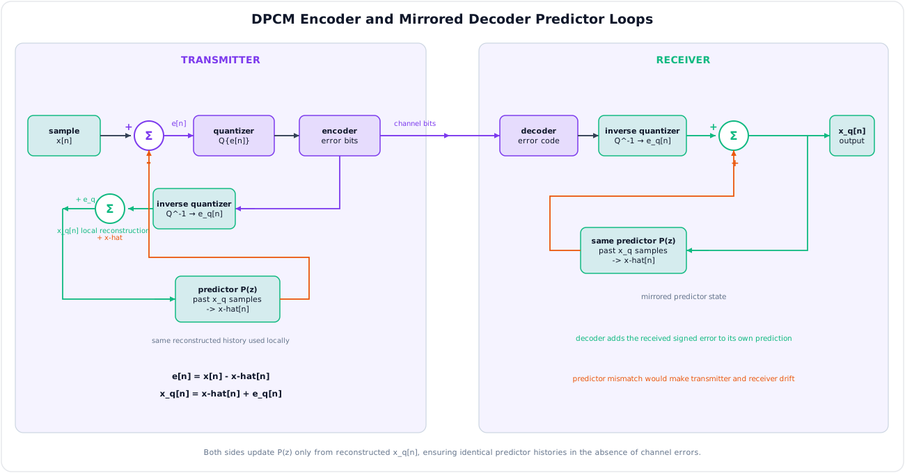
Let:
where \(\hat{x}[n]\) is the predicted sample. The quantized error is \(e_q[n]\), and the local reconstruction is:
The encoder must use the same reconstructed history as the decoder; otherwise their predictors drift apart.
Why DPCM Reduces Bit Rate
If prediction is effective, \(e[n]\) has lower variance and smaller dynamic range than \(x[n]\). It can therefore be quantized with fewer bits for comparable distortion.
DPCM Limitations
- Predictor complexity and state synchronization.
- Quantization error feeds the predictor loop.
- Channel errors may affect several later reconstructed samples until predictor memory decays.
- Poor prediction for rapidly changing or uncorrelated signals.
6. Adaptive Differential PCM (ADPCM)
ADPCM improves DPCM by adapting its quantizer step size, predictor coefficients or both according to recent signal behavior.
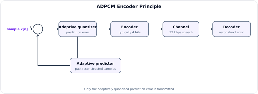
Operation
- Predict the current sample from past reconstructed samples.
- Subtract prediction from the actual input.
- Quantize the prediction error.
- Adapt the quantizer step: larger for rapidly changing signals, smaller for weak/slow signals.
- Update predictor parameters from reconstructed history.
- Transmit the compact error code.
- The decoder performs identical adaptation and adds the decoded error to its prediction.
Typical Speech Rate
ITU-T G.726 ADPCM supports rates including 16, 24, 32 and \(40\,\text{kbps}\). A commonly cited mode uses 4 bits/sample at \(8\,\text{kHz}\):
This is half the bit rate of 8-bit \(64\,\text{kbps}\) PCM, with useful telephony speech quality.
Advantages
- Lower bit rate and transmission bandwidth than PCM.
- Tracks changing speech amplitude better than fixed DPCM.
- Moderate computational complexity.
- Useful for speech storage, cordless telephony and legacy digital voice links.
ADPCM Limitations
- More complex and state-dependent than PCM.
- Channel errors can disturb adaptive state.
- Lower transparency for arbitrary high-quality audio.
- Encoder and decoder adaptation rules must match exactly.
PCM vs ADPCM
| Feature | PCM | ADPCM |
|---|---|---|
| Encoded quantity | Absolute quantized sample | Adaptive quantized prediction error |
| Typical telephone example | 8 bits/sample, \(64\,\text{kbps}\) | 4 bits/sample, \(32\,\text{kbps}\) |
| Predictor | None | Adaptive predictor |
| Quantizer | Uniform or companded | Adaptive step size |
| Complexity | Lower | Higher |
| Error propagation | Mostly one sample per corrupted word | May persist through predictor/adaptation state |
| Bandwidth | Higher | Lower for similar speech use |
| Robust general waveform quality | Better | Optimized mainly for correlated signals such as speech |
7. Delta Modulation and Adaptive Delta Modulation
Delta Modulation (DM)
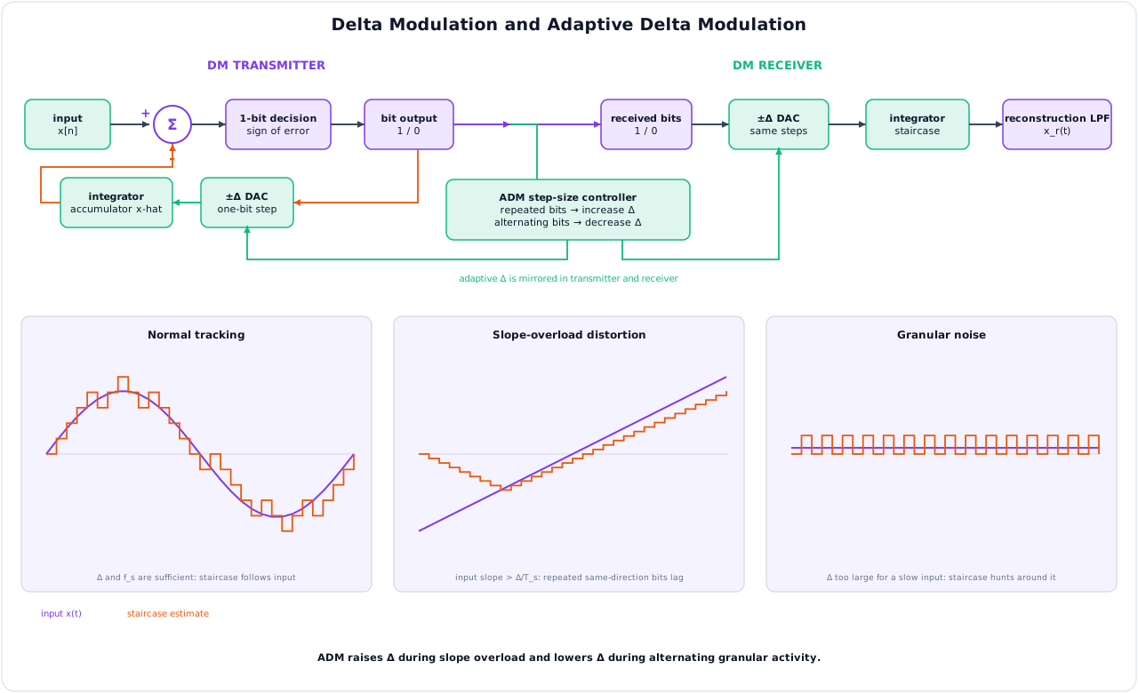
Delta modulation is a one-bit DPCM system. At every sampling instant, it sends only whether the local staircase estimate should rise or fall by fixed step \(\Delta\).
| Bit | Staircase update |
|---|---|
| 1 | Increase estimate by \(+\Delta\) |
| 0 | Decrease estimate by \(-\Delta\) |
The receiver integrates the one-bit sequence to reproduce the same staircase, then low-pass filters it.
Slope-Overload Distortion
The maximum staircase slope is approximately:
For \(x(t)=A_m\sin(2\pi f_m t)\), the maximum input slope is \(2\pi f_mA_m\). To track it:
If \(\Delta\) or \(f_s\) is too small, the staircase cannot follow a steep input and sustained slope overload occurs.
Granular Noise
When the input changes slowly and \(\Delta\) is too large, the staircase repeatedly jumps above and below the signal. This random-looking fluctuation is granular noise.
Fundamental Trade-Off
- Increase \(\Delta\) -> reduces slope overload but worsens granular noise.
- Decrease \(\Delta\) -> reduces granular noise but worsens slope overload.
- Increase \(f_s\) -> improves tracking but raises bit rate because DM sends one bit every sample.
Adaptive Delta Modulation (ADM)
ADM varies step size:
- Several identical consecutive bits indicate a steep slope -> increase \(\Delta\).
- Alternating bits indicate a slowly varying region -> decrease \(\Delta\).
This reduces both distortion mechanisms relative to a single fixed step.
8. Coder Comparison
| Feature | PCM | DPCM | ADPCM | Delta modulation |
|---|---|---|---|---|
| Encoded value | Absolute sample | Prediction error | Adaptive prediction error | Sign of one-step error |
| Bits/sample | Typically several | Fewer than PCM | Often 4 for speech | 1 |
| Required sample rate | Nyquist plus margin | Similar to PCM | Similar to PCM | Much higher (oversampling) |
| Complexity | Moderate | Predictor required | Adaptive predictor/quantizer | Simplest bit format, feedback integrator |
| Main impairment | Quantization noise | Prediction + quantization error | Adaptation/error propagation | Slope overload and granular noise |
| Typical use | General digital telephony/audio | Correlated waveform coding | Compressed telephony speech | Simple low-rate voice/control |
9. Key Exam Points
Key Exam Points - PCM and ADPCM
- PCM consists of sampling, quantization and encoding.
- Transmitter: LPF -> sampler/S&H -> quantizer -> encoder -> line coder.
- Receiver: regenerator -> line decoder -> code decoder/DAC -> reconstruction LPF.
- PCM bit rate: \(R_b=nf_s\); standard 8-bit, 8 kHz speech PCM is \(64\,\text{kbps}\).
- \(R_b/2\) is an ideal binary Nyquist lower bound, not every practical PCM line bandwidth.
- DPCM transmits prediction error; ADPCM also adapts predictor/quantizer.
- A common G.726 ADPCM mode is 4 bits/sample at \(8\,\text{kHz}=32\,\text{kbps}\).
- Delta modulation uses one bit/sample; small step causes slope overload and large step causes granular noise.
- ADM changes step size to reduce both DM impairments.
Model Answer — Generic PCM Transmitter and Receiver [10 marks, PYQ 2079]
Exam-ready answer
Pulse Code Modulation (PCM) represents each analog sample by an \(n\)-bit binary word. The complete system must preserve sampling, amplitude coding, bit timing and frame/channel position.
Part A — PCM transmitter [5 marks]
- Anti-aliasing LPF: limits message bandwidth to \(f_m<f_s/2\), preventing spectral replicas from overlapping after sampling.
- Sampler/sample-and-hold: takes uniform samples at \(f_s\geq2f_m\) and holds each value constant during quantization. For standard speech, \(f_s=8\,\text{kHz}\) and \(T_s=125\,\mu\text{s}\).
- Compressor, if used: A-law or \(\mu\)-law compresses speech dynamic range to improve low-level quantization performance.
- Quantizer: rounds the sample to one of \(L=2^n\) levels. For ideal span \(V_{FS}\), \(\Delta=V_{FS}/2^n\) and nearest-level error is approximately within \(\pm\Delta/2\).
- Encoder and serializer/line coder: assigns the selected level an \(n\)-bit word, serializes words, inserts framing/signaling as required, and produces a clock-recoverable physical waveform.
The uncoded single-channel payload rate is
Part B — PCM receiver [5 marks]
- Input filter/equalizer and 3R regenerator: limits noise/ISI, recovers clock, and re-amplifies, reshapes and retimes each line symbol by threshold decisions.
- Line decoder, de-framer and deserializer: removes the physical line code, finds frame/slot boundaries and reconstructs each \(n\)-bit sample word. Bit timing identifies bits; frame timing identifies channel positions.
- PCM decoder: maps each valid codeword back to its quantized amplitude. An expander applies the inverse A/\(\mu\) law when companding was used.
- DAC/hold: converts each word to an analog level and holds it for one sample period, producing a staircase/pulse waveform.
- Reconstruction LPF: passes the wanted baseband and suppresses sampling images/switching components before the destination.
The recovered waveform differs from the source by quantization error, filtering distortion and any uncorrected bit errors. For example, 8 bits/sample at \(8\,\text{kHz}\) gives \(64\,\text{kbps}\) before framing overhead. A significant-bit error can cause a much larger sample error than an LSB error, so regeneration and synchronization are essential.
Practice target: 16–18 minutes; divide time equally between the two five-mark chains and label clock, frame, companding and reconstruction paths.
Model Answer — PCM Principle and Advantages [5 marks]
Exam-ready answer
Pulse Code Modulation (PCM) is a digital waveform-coding method in which every uniformly timed analog sample is quantized and represented by a finite binary word. It has three defining operations: sampling discretizes time, quantization discretizes amplitude, and encoding assigns an \(n\)-bit code to one of \(2^n\) levels.
The transmitter uses anti-alias LPF \(\rightarrow\) S/H \(\rightarrow\) optional compressor \(\rightarrow\) quantizer \(\rightarrow\) encoder/line coder. Sampling must satisfy \(f_s\geq2f_m\) with practical guard band; the S/H keeps the input fixed during conversion. The receiver performs 3R regeneration and timing/frame recovery, decodes the word, applies optional expansion, converts it through a DAC/hold, and removes sampling images with a reconstruction LPF. The payload rate is
Advantages: threshold-based 3R repeaters prevent progressive analog noise accumulation; quality is reproducible over long links while decisions remain correct; PCM naturally supports TDM, digital switching and framing; binary data is easy to encrypt, store, process and protect with error-control coding; voice, data and signaling can share digital infrastructure; and IC implementation is stable and repeatable.
PCM is not cost-free. Finite levels create quantization noise, accurate bit/word/frame synchronization is required, and its bit stream commonly needs much more bandwidth than the original analog message. For standard telephone speech, \(n=8\) and \(f_s=8\,\text{kHz}\) give \(64\,\text{kbps}\) before framing. A-law/\(\mu\)-law companding improves weak-speech SQNR but does not eliminate quantization error. The complete five-mark answer should therefore state both the digital-regeneration benefit and the bandwidth/quantization trade-off.
Practice target: 8–9 minutes; define all three conversion operations, trace both directions, list five advantages and close with two limitations.
Model Answer — PCM Bit Rate, Ideal Bandwidth and SQNR [5 marks]
Exam-ready answer
Given sampling frequency \(f_s=8\,\text{kHz}\) and word length \(n=8\) bits/sample, the uncoded single-channel PCM payload rate is
For ideal two-level baseband signaling with zero intersymbol interference, Nyquist's pulse-transmission limit is \(R_b=2B\) bit/s. Therefore
This is a theoretical lower bound, not the bandwidth of every PCM line. Actual occupied bandwidth depends on line code, pulse shape, raised-cosine roll-off, equalization and the definition of bandwidth. Manchester coding needs more spectrum; framing and signaling raise the transmitted bit rate above the \(64\,\text{kbps}\) payload.
For an ideal uniform \(n\)-bit quantizer driven by a full-scale sinusoid, the quantization signal-to-noise ratio is
The assumptions matter: the error is modeled as uniformly distributed with power \(\Delta^2/12\), there is no clipping, jitter, thermal noise or nonlinearity, and the sine uses full scale. A signal backed off by \(A\,\text{dB}\) has approximately \(A\,\text{dB}\) lower uniform-quantizer SQNR. Telephone A/\(\mu\)-law companding deliberately changes SQNR versus input level, so \(49.92\,\text{dB}\) is not a universal measured speech-channel value.
Practice target: 7–8 minutes; show units on all three boxed results and state the signaling and full-scale-sine assumptions.
Model Answer — PCM, DPCM and ADPCM Comparison [10 marks]
Exam-ready answer
The three coders differ mainly in what is quantized. PCM sends an absolute sample; DPCM sends prediction error; ADPCM also changes predictor and/or quantizer parameters as signal statistics change.
PCM: sample \(x[n]\) is directly quantized and encoded. It needs no predictor and a conventional telephone example uses 8 bits/sample at \(8\,\text{kHz}\):
It is robust and transparent for general waveforms, but it ignores sample-to-sample correlation.
DPCM: the encoder predicts \(\hat{x}[n]\) from previous locally reconstructed samples and quantizes only
The encoder uses reconstructed, not original, past samples so its predictor state matches the decoder. Speech samples are correlated, so a good predictor makes \(\operatorname{var}(e)\) much smaller than \(\operatorname{var}(x)\). The smaller dynamic range can be represented by fewer bits for comparable distortion. Poor prediction, channel errors or rapidly changing inputs reduce this gain.
ADPCM: it retains the prediction-error loop but adapts quantizer step size, predictor coefficients or both from recent reconstructed data.
The sequence is predict \(\rightarrow\) subtract \(\rightarrow\) quantize error \(\rightarrow\) transmit compact code \(\rightarrow\) reconstruct \(\rightarrow\) update identical encoder/decoder states. Rapid or large errors increase step size to avoid overload; quiet intervals reduce it to lower granular quantization noise. A common ITU-T G.726 mode uses 4 bits/sample at \(8\,\text{kHz}\):
half the payload rate of 8-bit PCM for useful telephony speech quality.
| Feature | PCM | DPCM | ADPCM |
|---|---|---|---|
| Encoded quantity | Absolute quantized sample | Fixed-predictor error | Adaptively predicted/quantized error |
| Bits/sample | Usually highest | Lower if prediction works | Commonly 4 for speech, mode-dependent |
| Predictor/step | None; fixed/companded quantizer | Fixed predictor/quantizer | Predictor and/or step adapts |
| Complexity | Lowest | Moderate | Highest of the three |
| Error effect | Mainly corrupted sample word | May propagate through predictor memory | May disturb predictor and adaptive state |
| Best use | General telephony/audio | Correlated sources | Speech compression on rate-limited links |
At equal line coding/pulse shaping, lower \(R_b\) permits proportionally lower channel bandwidth. The saving is statistical, not lossless: ADPCM exploits correlation and accepts adaptive quantization/prediction distortion, more state complexity and possible error propagation. It performs less predictably on uncorrelated or high-fidelity arbitrary audio than on speech.
Practice target: 18–20 minutes; draw both feedback coders, write the prediction equations, calculate 64/32 kbps and reproduce the comparison table.
Model Answer — Delta Modulation, Slope Overload and Granular Noise [10 marks]
Exam-ready answer
Delta modulation (DM) is a one-bit predictive coder. At each high-rate sample it compares the input \(x[n]\) with a local staircase estimate \(x_q[n-1]\) and sends only the sign of the error. A 1 raises the estimate by fixed step \(\Delta\); a 0 lowers it:
The transmitter comparator produces the one-bit sequence and a feedback accumulator/integrator constructs the same staircase used for the next comparison. The receiver applies the bits to an identical accumulator and then low-pass filters the staircase. DM uses one bit/sample but normally samples far above the Nyquist rate, so its bit rate is \(R_b=f_s\) rather than necessarily being small.
Slope-overload distortion: the staircase can change by only \(\Delta\) in one period \(T_s\), so its maximum tracking slope is
For \(x(t)=A_m\sin(2\pi f_m t)\), the maximum source slope is \(2\pi f_mA_m\). Avoiding sustained overload requires approximately
If \(\Delta\) or \(f_s\) is too small, long runs of identical bits command the steepest staircase but it still falls behind the waveform.
Granular noise: when the input is nearly constant or changes slowly and \(\Delta\) is too large, the estimate repeatedly jumps above and below it. Alternating up/down bits create a grain-like fluctuation. Decreasing \(\Delta\) reduces this error but worsens slope overload, giving the fixed-step trade-off.
Numerical check: for \(A_m=1\,\text{V}\), \(f_m=1\,\text{kHz}\) and \(f_s=32\,\text{kHz}\),
A fixed \(0.10\,\text{V}\) step can supply only \(3200\,\text{V/s}\) against the required \(6283\,\text{V/s}\) and will overload near the steepest crossing. A \(0.25\,\text{V}\) step can track that slope but may chatter badly on flat portions.
Adaptive delta modulation (ADM) resolves much of the conflict by varying \(\Delta[n]\). Several identical consecutive bits indicate sustained slope, so the controller increases the step; alternating bits indicate a slowly varying region, so it decreases the step. Both transmitter and receiver apply the same update rule to remain synchronized. ADM reduces, but cannot completely eliminate, overload and granular error; channel bit errors can also perturb the adaptive state.
Practice target: 18–20 minutes; draw both feedback accumulators, derive the slope condition with units, sketch both errors and solve one minimum-step example.
Model Answer — PCM versus ADPCM [5 marks]
Exam-ready answer
PCM and ADPCM are waveform coders, but PCM quantizes absolute sample amplitude whereas ADPCM quantizes a smaller, adaptively scaled prediction error.
| Basis | PCM | ADPCM |
|---|---|---|
| Principle | Sample, quantize and encode \(x[n]\) directly | Predict \(\hat{x}[n]\), encode \(e[n]=x[n]-\hat{x}[n]\), adapt predictor/step |
| Typical speech example | 8 bits/sample at 8 kHz = \(64\,\text{kbps}\) | G.726 4 bits/sample at 8 kHz = \(32\,\text{kbps}\), with other rates available |
| Bandwidth | Higher for the same line code/pulse shape | Lower roughly in proportion to bit rate |
| Circuit/algorithm | Simpler, no prediction state | More computation and matched encoder/decoder state |
| Noise/distortion | Absolute-sample quantization; companding optional | Prediction plus adaptive quantization distortion |
| Channel error | Often one sample is badly wrong, especially after MSB error | May propagate through predictor and adaptation memory |
| Application | General digital telephony, audio, measurement | Rate-limited speech storage, cordless/legacy voice links |
ADPCM saves rate because adjacent speech samples are correlated. If prediction is good, \(\operatorname{var}(e)\ll\operatorname{var}(x)\), so fewer quantizer bits can describe the error with useful speech quality. At \(8\,\text{kHz}\) the common 4-bit example halves payload rate from 64 to \(32\,\text{kbps}\); under ideal two-level Nyquist signaling its lower-bound bandwidth correspondingly changes from 32 to \(16\,\text{kHz}\). Those bandwidth values exclude framing and depend on signaling assumptions.
PCM is simpler, more robust to state disturbance and more transparent for arbitrary signals. ADPCM is more bandwidth-efficient for correlated speech but is state-dependent, can propagate channel errors and may perform poorly when the signal changes unpredictably. The lower rate is therefore achieved by exploiting source redundancy, not by carrying the same absolute samples losslessly.
Practice target: 8–9 minutes; reproduce the seven comparison rows, the prediction equation and the 64-to-32 kbps calculation.