Antennas and Waveguides
Possible Exam Questions
Exam Questions and Answer Map
Questions labelled [PYQ paper/year] are observed past questions; those labelled [likely] are pattern-based predictions. For each one, rehearse the answer plan closed-book, then use the links to verify the full answer in this chapter.
-
Explain antenna fundamentals; define radiation pattern, directivity, gain and efficiency. [5–10] — [likely]
-
Answer plan: Define antenna → list key parameters (radiation pattern, beamwidth, directivity, gain, efficiency, radiation resistance) → write \(G = \eta_{\text{rad}} D\) → define effective aperture → draw a sample radiation pattern showing lobes.
-
Model answer: Antenna fundamentals and radiation parameters
-
Discuss the working principle and radiation characteristics of a half-wave dipole antenna. [5] — [PYQ 2082]
-
Answer plan: Describe half-wave dipole geometry (\(l=\lambda/2\)) → state current distribution (sinusoidal, max at center) → give radiation resistance \(R_r \approx 73\,\Omega\) → describe doughnut radiation pattern → state directivity \(D=1.64\) (2.15 dBi).
-
Model answer: Half-wave dipole operation and radiation
-
Explain polarization and impedance matching in antenna systems. [5] — [PYQ 2082]
-
Answer plan: Define polarization (orientation of \(\vec E\)) → describe linear, circular, elliptical types → explain polarization loss factor → define input impedance → state matching condition for max power transfer.
-
Model answer: Antenna polarization and impedance matching
-
Mention the types of antenna used in the VHF band; how can you increase the gain of such an antenna? Is a parabolic antenna feasible in the VHF band? [2+6+2=10] — [PYQ 2079]
-
Answer plan: List VHF antennas (dipole, Yagi-Uda, folded dipole) → explain gain increase methods (add directors, increase boom length, use arrays) → explain why parabolic dish is impractical at VHF (huge dish needed since \(D\propto (d/\lambda)^2\) and \(\lambda\) is large at VHF).
-
Model answer: VHF antennas, gain improvement, and dish feasibility
-
Explain waveguides; why do they act as high-pass filters? Define the dominant mode. [5–10] — [likely]
-
Answer plan: Define waveguide → explain cutoff frequency \(f_c\) (below which no propagation) → derive \(f_c\) for rectangular waveguide → explain why this creates HPF behavior → define dominant mode (lowest \(f_c\) mode: TE₁₀ for rectangular).
- Model answer: Rectangular waveguide cutoff and dominant TE10 mode
Syllabus Focus
- Antenna fundamentals
- Polarizations
- Radiation from dipole antenna
- Waveguides
1. Antenna Fundamentals
Likely Exam Question (5 marks)
"Define antenna. Explain important antenna parameters such as radiation pattern, directivity, gain, beamwidth, and radiation resistance."
An antenna is a transducer that converts electrical signals into electromagnetic waves during transmission and electromagnetic waves into electrical signals during reception.
In a transmitter:
In a receiver:
Why Antennas Radiate
Radiation occurs when charges are accelerated or currents vary with time.
- A DC current in an ideal straight wire does not radiate significantly.
- A time-varying current produces time-varying electric and magnetic fields.
- These fields detach from the antenna and propagate as electromagnetic waves.
For efficient radiation, antenna dimensions are usually comparable to wavelength, commonly \(\lambda/4\) or \(\lambda/2\).
Basic Antenna Parameters
| Parameter | Meaning |
|---|---|
| Radiation pattern | Angular distribution of radiated power or field |
| Beamwidth | Angular width of main lobe between specified power points |
| Directivity | Ability to concentrate radiation in a particular direction |
| Gain | Directivity including antenna efficiency |
| Radiation resistance | Equivalent resistance representing radiated power |
| Input impedance | Impedance seen at antenna terminals |
| Bandwidth | Frequency range over which antenna performs satisfactorily |
| Polarization | Orientation of the radiated electric field |
| Effective aperture | Effective area that captures power from an incident wave |
2. Radiation Pattern
Likely Exam Question (5 marks)
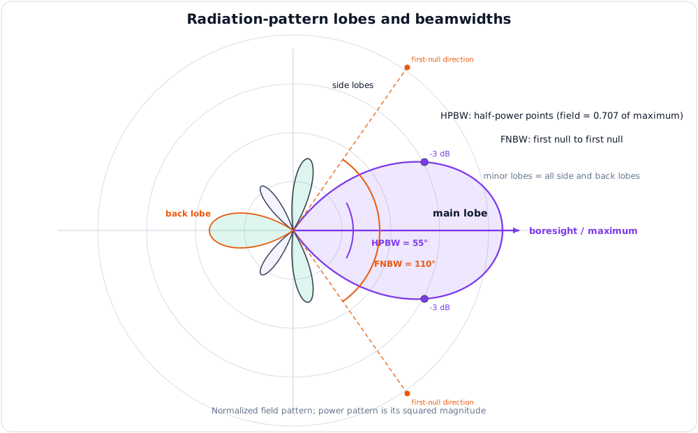
"What is an antenna radiation pattern? Explain main lobe, side lobe, back lobe, HPBW, and FNBW."
The radiation pattern of an antenna is a graphical representation of the radiation properties of the antenna as a function of direction.
It may represent:
- Electric field intensity \(E\)
- Magnetic field intensity \(H\)
- Power density \(S\)
- Radiation intensity \(U\)
Types of Radiation Pattern
| Pattern Type | Description |
|---|---|
| Field pattern | Plot of \(\lvert E\rvert\) or \(\lvert H\rvert\) versus direction |
| Power pattern | Plot of power density or radiation intensity versus direction |
| 2D pattern | Pattern in one principal plane, such as E-plane or H-plane |
| 3D pattern | Full spatial distribution |
Lobes
| Term | Meaning |
|---|---|
| Main lobe | Lobe containing direction of maximum radiation |
| Side lobes | Smaller lobes in undesired directions |
| Back lobe | Lobe approximately opposite to main lobe |
| Minor lobes | All lobes except main lobe |
Side lobes and back lobes usually represent wasted power and possible interference.
Beamwidth
Half-Power Beamwidth (HPBW): angular separation between two points on the main lobe where power falls to half of maximum value.
Half power corresponds to:
or field magnitude:
First-Null Beamwidth (FNBW): angular separation between the first nulls on either side of the main lobe.
Generally:
Isotropic, Omnidirectional, and Directional Antennas
| Antenna Type | Description |
|---|---|
| Isotropic | Hypothetical antenna radiating equally in all directions |
| Omnidirectional | Uniform radiation in one plane, directional in another |
| Directional | Concentrates radiation in one or more preferred directions |
An isotropic antenna cannot be physically realized but is used as a reference.
3. Radiation Intensity, Directivity, Gain, and Efficiency
Likely Exam Question (10 marks)
"Define directivity, gain, efficiency, and effective aperture of an antenna. Derive their relationships."
Radiation Intensity
Radiation intensity is power radiated per unit solid angle.
Unit: W/sr
Total radiated power:
For an isotropic radiator:
Directivity
Directivity is the ratio of maximum radiation intensity to average radiation intensity.
Since \(U_{\text{avg}} = P_{\text{rad}}/(4\pi)\):
For isotropic antenna:
Approximate directivity in terms of beam solid angle \(\Omega_A\):
If HPBW values are given in degrees for two principal planes:
where \(\theta_{\text{HP}}\) and \(\phi_{\text{HP}}\) are in degrees.
Gain
Gain is directivity multiplied by radiation efficiency.
where \(\eta_r\) is radiation efficiency.
In decibels:
When referenced to isotropic antenna:
When referenced to half-wave dipole:
Radiation Efficiency
Radiation efficiency is the ratio of radiated power to input power accepted by the antenna.
If antenna has radiation resistance \(R_r\) and loss resistance \(R_l\):
Effective Aperture
Effective aperture is the effective area of a receiving antenna that captures power from an incident wave.
where:
- \(P_r\) = received power
- \(S\) = incident power density
Relation between gain and effective aperture:
or:
4. Radiation Resistance and Input Impedance
Radiation Resistance
Radiation resistance is a fictitious resistance that would dissipate the same amount of power as the antenna radiates.
If antenna current is \(I_{\text{rms}}\):
Using peak current \(I_0\):
Radiation resistance is not a physical resistor; it represents useful radiated power.
Input Impedance
Antenna input impedance is:
where:
For maximum power transfer, antenna input impedance should be matched to the transmission line impedance.
Common practical target:
5. Polarization
Likely Exam Question (5 or 10 marks)
"Define polarization of an antenna. Explain linear, circular, and elliptical polarization."
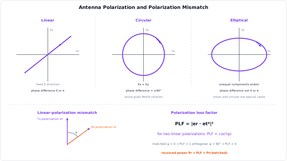
Polarization of an electromagnetic wave is the orientation of the electric field vector as the wave propagates.
The polarization of an antenna is the polarization of the wave it radiates in the far-field region.
Linear Polarization
In linear polarization, the electric field remains along a fixed straight line.
Examples:
- Vertical polarization: \(\vec E\) is vertical.
- Horizontal polarization: \(\vec E\) is horizontal.
If the electric field is:
then polarization is linear along \(x\).
Circular Polarization
In circular polarization, the tip of the electric field vector traces a circle as time progresses.
Conditions for circular polarization:
- Two perpendicular electric-field components have equal magnitudes.
- Phase difference between them is \(90^\circ\).
Example:
Types:
| Type | Description |
|---|---|
| RHCP | Right-hand circular polarization |
| LHCP | Left-hand circular polarization |
Circular polarization is widely used in satellite communication because it reduces sensitivity to antenna orientation.
Elliptical Polarization
In elliptical polarization, the tip of the electric field vector traces an ellipse.
It occurs when:
- Perpendicular components have unequal magnitudes, or
- Phase difference is not exactly \(0^\circ\), \(180^\circ\), or \(90^\circ\) with equal magnitudes.
Linear and circular polarizations are special cases of elliptical polarization.
Polarization Loss
Maximum received power occurs when transmitting and receiving antennas have the same polarization.
Polarization loss factor:
where:
- \(\hat e_t\) = transmitted wave polarization unit vector
- \(\hat e_r\) = receiving antenna polarization unit vector
For two linearly polarized antennas with angle \(\psi\) between their polarizations:
Special cases:
| Polarization Mismatch | \(PLF\) |
|---|---|
| Same polarization | \(1\) |
| \(45^\circ\) mismatch | \(0.5\) |
| Orthogonal polarization | \(0\) |
6. Radiation from Dipole Antenna
Likely Exam Question (10 marks)
"Explain radiation from a short dipole and half-wave dipole. State radiation pattern, radiation resistance, and important characteristics."
A dipole antenna consists of two conducting arms fed at the center by a transmission line.
Hertzian Dipole
A Hertzian dipole is an ideal infinitesimal current element with length \(l \ll \lambda\) and uniform current distribution.
It is mainly a theoretical antenna used to derive radiation fields.
Far-field components are:
Thus:
Power pattern:
Properties:
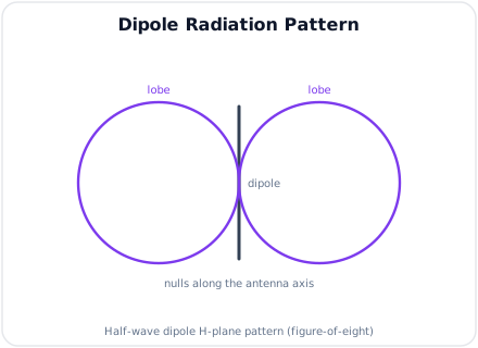
- Maximum radiation at \(\theta = 90^\circ\) broadside to the dipole.
- Zero radiation along the dipole axis, \(\theta = 0^\circ\) and \(180^\circ\).
- Radiation pattern is doughnut-shaped in 3D.
Radiation resistance of a Hertzian dipole:
Short Dipole
A short dipole has length \(l \ll \lambda\), but current is triangular rather than uniform.
Radiation resistance:
Short dipoles have low radiation resistance, so they are inefficient unless loss resistance is very small.
Half-Wave Dipole
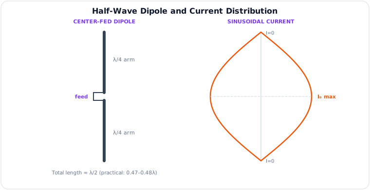
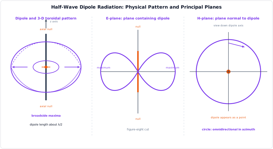
A half-wave dipole has total length approximately:
In practice, physical length is slightly less than \(\lambda/2\) due to end effects:
Current distribution is approximately sinusoidal:
where \(z=0\) at the center and endpoints are near \(z=\pm\lambda/4\).
Properties of half-wave dipole:
| Parameter | Approximate Value |
|---|---|
| Radiation resistance | \(73\,\Omega\) |
| Directivity | \(1.64\) |
| Gain reference | \(2.15\,\text{dBi}\) |
| HPBW | about \(78^\circ\) |
| Pattern | Omnidirectional in azimuth, figure-eight in elevation |
The half-wave dipole is a common practical reference antenna.
VHF Antennas and Gain Improvement (NTC 2079)
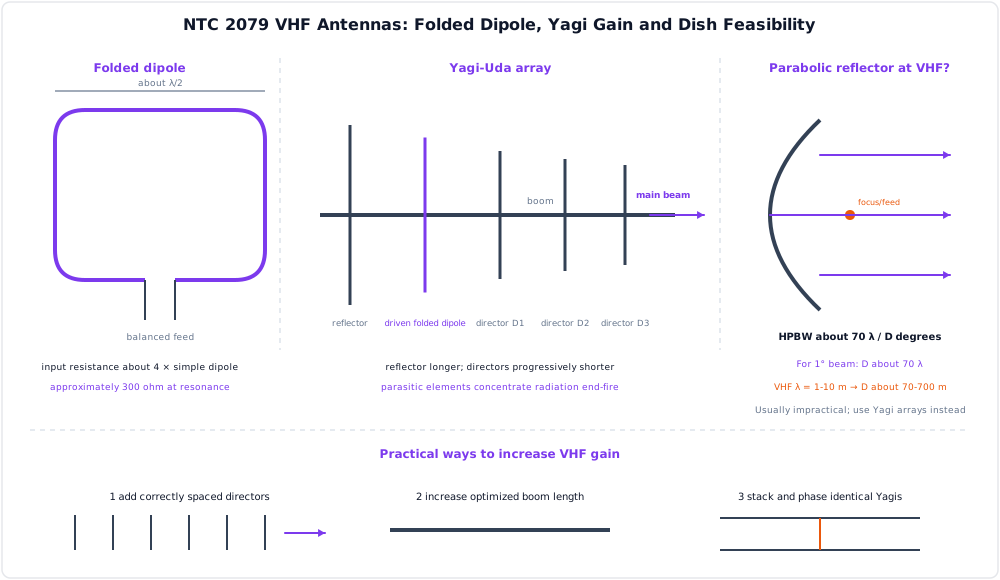
Common VHF antennas include the half-wave dipole, folded dipole, Yagi-Uda array, log-periodic array and collinear array. A folded dipole has approximately four times the feed resistance of a simple dipole. A Yagi increases end-fire gain by using a longer reflector behind the driven element and one or more shorter directors in front.
Practical gain improvements are to add correctly spaced directors, optimize/increase boom length, and stack identical Yagis with the correct spacing and phase. For a parabolic reflector,
so a narrow VHF beam requires an extremely large diameter because \(\lambda\) is large at VHF. A dish is therefore normally impractical compared with a Yagi or stacked array.
Monopole Antenna
A quarter-wave monopole is equivalent to half of a dipole placed above a conducting ground plane.
Approximate radiation resistance:
It radiates only in the upper half-space, so its directivity is twice that of a half-wave dipole over perfect ground.
7. Antenna Regions
Likely Exam Question (5 marks)
"Differentiate between near-field and far-field regions of an antenna."
The field around an antenna is divided into regions based on distance from the antenna.
Reactive Near Field
This region is very close to the antenna. Stored electric and magnetic energies dominate.
Approximate boundary for a small antenna:
where \(D\) is the largest antenna dimension.
Radiating Near Field or Fresnel Region
Radiating fields dominate, but angular field distribution still depends on distance.
Approximate region:
Far Field or Fraunhofer Region
Radiation pattern is essentially independent of distance.
Far-field condition:
In the far field:
- \(\vec E\) and \(\vec H\) are transverse to direction of propagation.
- \(E/H = \eta\).
- Power density varies approximately as \(1/r^2\).
- Radiation pattern measurements are normally made in this region.
8. Friis Transmission Equation
Likely Exam Question (5 marks)
"State Friis transmission equation and explain its significance in antenna communication links."
Friis transmission equation gives received power in free space between two matched antennas in the far field.
where:
- \(P_t\) = transmitted power
- \(P_r\) = received power
- \(G_t\) = transmit antenna gain
- \(G_r\) = receive antenna gain
- \(R\) = separation distance
- \(\lambda\) = wavelength
In decibel form:
Free-space path loss:
In dB:
For \(R\) in km and \(f\) in MHz:
9. Waveguides
Likely Exam Question (10 marks)
"What is a waveguide? Explain TE and TM modes, cutoff frequency, guide wavelength, and dominant mode in a rectangular waveguide."
A waveguide is a hollow conducting structure used to guide electromagnetic waves, usually at microwave frequencies.
Unlike two-wire or coaxial lines, waveguides generally support waves only above a cutoff frequency.
Why Waveguides Are Used
- Low loss at microwave frequencies.
- High power-handling capability.
- No radiation leakage if properly constructed.
- Useful for radar, satellite, microwave links, and RF test systems.
Waveguide Types
| Type | Description |
|---|---|
| Rectangular waveguide | Most common, simple analysis, dominant TE\(_{10}\) mode |
| Circular waveguide | Used where rotation symmetry is useful |
| Ridged waveguide | Wider bandwidth than ordinary rectangular waveguide |
| Dielectric waveguide | Guides waves using dielectric boundaries |
10. Modes in Waveguides
Waveguide modes are field patterns that can propagate along the guide.
TEM Mode
TEM means transverse electromagnetic:
TEM waves require at least two conductors, such as coaxial or parallel-wire lines.
Hollow rectangular waveguides cannot support TEM mode because they have only one conducting boundary.
TE Mode
TE means transverse electric:
The electric field has no component in the direction of propagation, but magnetic field has a longitudinal component.
TE modes are written as TE\(_{mn}\).
TM Mode
TM means transverse magnetic:
The magnetic field has no component in the direction of propagation, but electric field has a longitudinal component.
TM modes are written as TM\(_{mn}\).
Mode Indices
For rectangular waveguide TE\(_{mn}\) or TM\(_{mn}\):
- \(m\) = number of half-wave variations across wider dimension \(a\).
- \(n\) = number of half-wave variations across narrower dimension \(b\).
For TM modes, both \(m\) and \(n\) must be nonzero.
For TE modes, either \(m\) or \(n\) may be zero, but not both.
11. Rectangular Waveguide
Consider a rectangular waveguide with dimensions:
where:
- \(a\) = broader wall dimension
- \(b\) = narrower wall dimension
Cutoff Wavelength
For TE\(_{mn}\) or TM\(_{mn}\) mode:
Cutoff Frequency
For a waveguide filled with medium of velocity \(v = 1/\sqrt{\mu\epsilon}\):
For air-filled waveguide:
Propagation occurs only if:
If \(f < f_c\), the mode is evanescent and decays along the guide.
Dominant Mode
The dominant mode is the mode with the lowest cutoff frequency.
For a rectangular waveguide with \(a > b\), the dominant mode is:
For TE\(_{10}\):
The TE\(_{10}\) mode is dominant because it has the largest cutoff wavelength and therefore the lowest cutoff frequency.
Guide Wavelength
Guide wavelength is the distance along the waveguide over which phase changes by \(2\pi\).
where \(\lambda\) is wavelength in the filling medium.
Since \(\lambda < \lambda_c\) for propagation:
Phase and Group Velocity
Phase velocity in a waveguide:
Group velocity:
Relationship:
For air-filled waveguide:
Phase velocity can exceed \(c\), but this does not violate relativity because information and energy travel with group velocity, which is less than \(c\).
Wave Impedance in Waveguides
For TE modes:
For TM modes:
where \(\eta\) is intrinsic impedance of the filling medium.
12. Rectangular Waveguide TE10 Mode
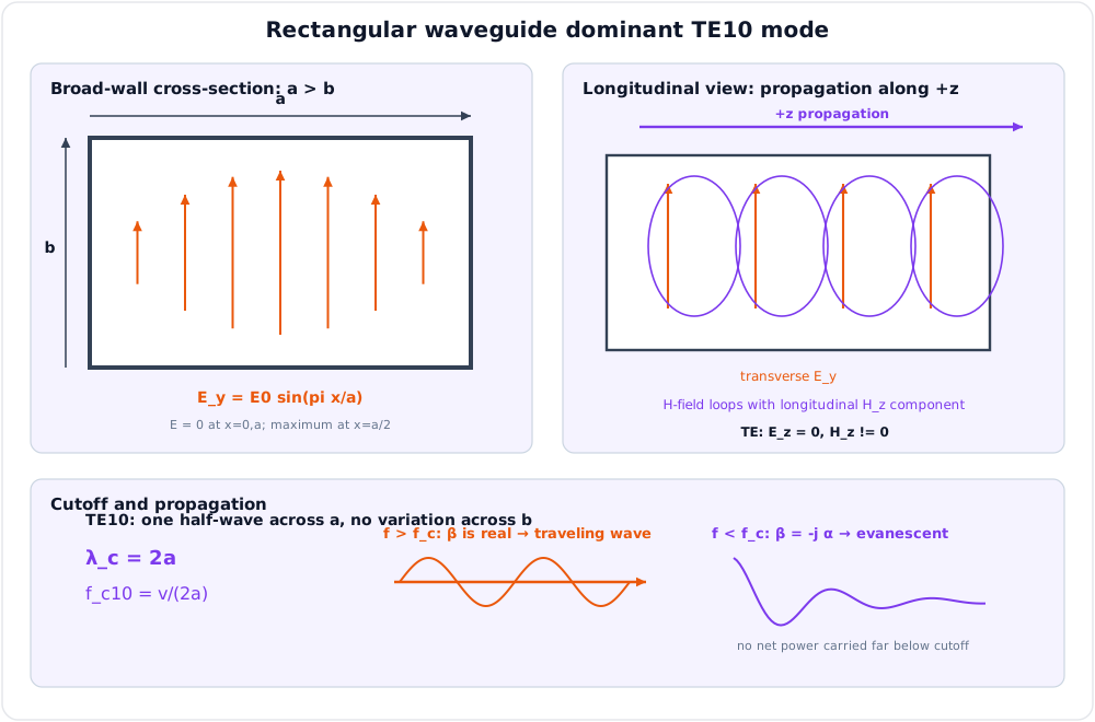
For the dominant TE\(_{10}\) mode:
- There is one half-wave variation across the broad dimension \(a\).
- There is no variation across the narrow dimension \(b\).
- \(E_z = 0\) and \(H_z \ne 0\).
Cutoff frequency:
Cutoff wavelength:
Guide wavelength:
TE\(_{10}\) field properties:
- Electric field is maximum at the center of the broad wall.
- Electric field is zero at the conducting side walls.
- Power flows along the guide axis.
- It is the preferred mode for single-mode waveguide operation.
Single-Mode Operation
For rectangular waveguide, single-mode operation means only TE\(_{10}\) propagates while higher modes are below cutoff.
The operating frequency should satisfy:
For many rectangular guides with \(a \approx 2b\), the next higher modes are TE\(_{20}\) and TE\(_{01}\).
13. Waveguide Advantages and Limitations
Advantages
- Lower conductor loss than coaxial cable at microwave frequencies.
- Can handle high power.
- Good shielding and low radiation leakage.
- High Q-factor for resonant components.
Limitations
- Bulky at low frequencies because size is proportional to wavelength.
- Cannot propagate below cutoff frequency.
- Narrower bandwidth than coaxial lines in many applications.
- Bends, joints, and discontinuities can cause reflections.
- More expensive and mechanically rigid.
Applications
- Radar transmitters and receivers
- Microwave communication links
- Satellite earth stations
- Microwave ovens
- RF measurement systems
- Antenna feed networks
14. Solved Examples
Example 1 - Dipole Length
Q. Find the approximate length of a half-wave dipole for \(100\,\text{MHz}\).
Solution:
Ideal half-wave length:
Practical length:
Example 2 - Antenna Gain from Directivity and Efficiency
Q. An antenna has directivity \(D = 8\) and radiation efficiency \(70\%\). Find gain in linear scale and dBi.
Solution:
Example 3 - Polarization Loss
Q. Two linearly polarized antennas have a polarization mismatch angle of \(30^\circ\). Find polarization loss factor.
Solution:
Thus, 75% of the power is received due to polarization matching, ignoring other losses.
Example 4 - Rectangular Waveguide Cutoff Frequency
Q. An air-filled rectangular waveguide has broad dimension \(a = 4\,\text{cm}\). Find the cutoff frequency for TE\(_{10}\) mode.
Solution:
Example 5 - Guide Wavelength
Q. An air-filled rectangular waveguide has TE\(_{10}\) cutoff frequency \(6\,\text{GHz}\). Find guide wavelength at \(10\,\text{GHz}\).
Solution:
Free-space wavelength:
Cutoff wavelength:
Guide wavelength:
Example 6 - Friis Transmission
Q. A transmitter radiates \(10\,\text{W}\) at \(1\,\text{GHz}\) using antennas with \(G_t = 10\) and \(G_r = 5\). Distance is \(1\,\text{km}\). Find received power in free space.
Solution:
or approximately:
15. Quick Revision Table
| Topic | Key Result |
|---|---|
| Antenna | Converts guided electrical signal to radiated EM wave and vice versa |
| Radiation intensity | \(U = r^2S_{\text{rad}}\) |
| Directivity | \(D = 4\pi U_{\max}/P_{\text{rad}}\) |
| Gain | \(G = \eta_rD\) |
| Effective aperture | \(A_e = G\lambda^2/(4\pi)\) |
| Radiation resistance | \(P_{\text{rad}} = I_{\text{rms}}^2R_r\) |
| Polarization loss | \(PLF = \lvert\hat e_t\cdot\hat e_r\rvert^2\) |
| Hertzian dipole pattern | \(P(\theta) \propto \sin^2\theta\) |
| Hertzian dipole resistance | \(R_r = 80\pi^2(l/\lambda)^2\) |
| Short dipole resistance | \(R_r = 20\pi^2(l/\lambda)^2\) |
| Half-wave dipole resistance | \(R_r \approx 73\,\Omega\) |
| Friis equation | \(P_r = P_tG_tG_r(\lambda/4\pi R)^2\) |
| Rectangular waveguide cutoff | \(f_c = \frac{c}{2}\sqrt{(m/a)^2+(n/b)^2}\) |
| Dominant rectangular mode | TE\(_{10}\) |
| TE\(_{10}\) cutoff | \(f_c = c/(2a)\) |
| Guide wavelength | \(\lambda_g = \lambda/\sqrt{1-(\lambda/\lambda_c)^2}\) |
| TE wave impedance | \(Z_{TE}=\eta/\sqrt{1-(f_c/f)^2}\) |
| TM wave impedance | \(Z_{TM}=\eta\sqrt{1-(f_c/f)^2}\) |
Key Exam Points - Antennas and Waveguides
- Antenna polarization is defined by the electric field orientation, not magnetic field orientation.
- Half-wave dipole has radiation resistance about \(73\,\Omega\) and gain \(2.15\,\text{dBi}\).
- Maximum dipole radiation is broadside; zero radiation is along the dipole axis.
- Hollow rectangular waveguides support TE and TM modes, but not TEM mode.
- TE\(_{10}\) is the dominant mode of a rectangular waveguide because it has the lowest cutoff frequency.
- Waveguides propagate only above cutoff frequency.
Model Answer — Antenna Fundamentals and Radiation Parameters [10 marks]
Exam-ready answer
An antenna is a reciprocal electromagnetic transducer: in transmission it converts a guided voltage/current wave into a radiated wave, and in reception it converts incident electromagnetic power into a guided signal. In the far field, take \(\hat a_r\) radially outward from the antenna; \(\vec E\) and \(\vec H\) are transverse and the average Poynting vector \(\langle\vec S\rangle=\tfrac12\operatorname{Re}(\vec E\times\vec H^*)\) points along \(+\hat a_r\).
Radiation pattern is the angular variation of field or power at fixed large \(r\), normally normalized to its maximum. A pattern identifies the main lobe, side lobes, back lobe and nulls. The half-power beamwidth (HPBW) is the angle between points where power is half its maximum, equivalent to field magnitude \(1/\sqrt2\) of maximum; first-null beamwidth is measured between the first nulls around the main lobe.
At distance \(r\), radiation intensity is power per unit solid angle:
An isotropic reference radiates \(U_0=P_{\rm rad}/4\pi\). Directivity compares radiation in a direction with that reference and depends only on pattern shape:
Radiation efficiency accounts for conductor and dielectric loss:
Gain includes this loss, so
Realized gain additionally includes mismatch loss \(1-|\Gamma|^2\). Radiation resistance \(R_r\) is the equivalent resistance that would dissipate the radiated power: \(P_{\rm rad}=I_{\rm rms}^2R_r\). The terminal impedance is \(Z_A=R_r+R_{\rm loss}+jX_A\) ohms.
In reception, effective aperture is \(A_e=P_{\rm available}/S_{\rm inc}\) in m\(^2\). For matched polarization and impedance,
This connects transmitting gain to receiving capture area. Polarization mismatch multiplies received power by \(|\hat e_r^*\cdot\hat e_t|^2\).
Worked check: if \(D_0=6\), \(\eta_{\rm rad}=0.75\) and \(\lambda=1\) m, then \(G_0=4.5=6.53\) dBi and \(A_{e,\max}=4.5/(4\pi)=0.358\) m\(^2\). Directivity can be high even for a lossy antenna, whereas gain falls with loss; a narrow beam generally means larger directivity.
These parameters govern link budgets, radar, broadcasting and direction finding. They assume far-field observation and a stated polarization/reference; near fields, nearby ground, feeder loss and mismatch can substantially change measured performance, so gain must not be inferred from beamwidth alone without an applicable pattern model.
Practice target: 18 minutes; draw and label the pattern, then derive the D-G-efficiency-aperture chain with units.
Model Answer — Half-Wave Dipole Operation and Radiation [5 marks]
Exam-ready answer
A half-wave dipole is a balanced, centre-fed straight conductor with total electrical length \(l\simeq\lambda/2\), consisting of two approximately \(\lambda/4\) arms. Let it lie on the \(z\)-axis, with spherical angle \(\theta\) measured from \(+z\) and outward propagation along \(\hat a_r\). The RF source drives opposite charges and currents on the two arms. The thin-wire current is approximately sinusoidal,
so current is maximum at the feed point and zero at the open ends.
For an ideal thin half-wave element, the far electric field has \(\hat a_\theta\) polarization and angular factor
Thus \(\vec E\times\vec H\) points radially outward. Radiation is maximum broadside at \(\theta=90^\circ\) and zero along the wire at \(\theta=0^\circ,180^\circ\). The E-plane, containing the dipole axis, is a figure eight; the H-plane, perpendicular to the axis, is a circle. The three-dimensional pattern is a torus.
Its ideal radiation resistance is about \(73\,\Omega\), directivity is \(D_0=1.64=2.15\) dBi, and polarization is linear parallel to the dipole. An exactly \(0.5\lambda\) thin dipole has a small inductive reactance; shortening it to roughly \(0.47\)-\(0.48\lambda\) commonly makes the practical element resonant, depending on diameter and environment.
Check: at \(100\) MHz, \(\lambda=c/f=3\) m, so the ideal total length is \(1.5\) m and each arm is \(0.75\) m; a practical resonant length is about \(1.44\) m before final tuning. The dipole is simple, reciprocal and a reference for antenna gain, but it requires a balanced feed or balun, has modest gain, and is detuned by conductor thickness, ground and nearby objects.
Practice target: 9 minutes; draw the current distribution and both principal-plane cuts, with broadside maximum and axial nulls.
Model Answer — Antenna Polarization and Impedance Matching [5 marks]
Exam-ready answer
Polarization is the locus and orientation traced by the electric-field vector at a fixed point as time advances; it is defined by \(\vec E\), not \(\vec H\). For propagation along \(+z\), write orthogonal components using the \(e^{j\omega t}\) convention:
- Linear: \(\delta=0\) or \(\pi\), or one component is zero; the tip of \(\vec E\) follows a line.
- Circular: \(|E_x|=|E_y|\) and \(|\delta|=90^\circ\); the magnitude is constant and the tip follows a circle.
- Elliptical: the general unequal-amplitude or other-phase case; linear and circular are special cases.
Handedness must be stated with a viewing convention because reversing the observation direction reverses the apparent rotation.
The receiving antenna extracts the component aligned with its polarization. For normalized complex polarization vectors,
and for two linear polarizations separated by angle \(\psi\), \(\mathrm{PLF}=\cos^2\psi\). Orthogonal ideal polarizations give zero received power.
For impedance matching, represent antenna input impedance as
Maximum available power from the antenna occurs with conjugate load matching, \(Z_L=Z_A^*\). For a real transmission line of characteristic impedance \(Z_0\), the usual design target is a resonant transformed antenna input \(Z_{in}=Z_0\), giving
Matching networks, baluns, stubs or quarter-wave transformers cancel reactance and transform resistance; they do not repair polarization mismatch.
Check: a \(30^\circ\) linear-polarization error gives PLF \(=\cos^230^\circ=0.75\), a \(1.25\) dB loss, even with perfect impedance matching. Conversely, an impedance match cannot recover power rejected by orthogonal polarization. Matching improves delivered/received power and protects transmitters, but practical networks have loss and finite bandwidth; polarization can also vary through multipath or Faraday rotation.
Practice target: 9 minutes; define polarization from E, write the complex-vector PLF, then distinguish conjugate and line matching.
Model Answer — VHF Antennas, Gain Improvement, and Dish Feasibility [10 marks]
Exam-ready answer
Part A — Suitable VHF antennas [2 marks]
VHF covers \(30\)-\(300\) MHz, corresponding approximately to \(\lambda=10\)-\(1\) m. Common antennas are the half-wave dipole, folded dipole, quarter-wave ground-plane/monopole, Yagi-Uda, log-periodic array, collinear array and turnstile/crossed dipoles. Dipoles and folded dipoles are useful driven elements; a Yagi gives a directional fixed-frequency beam, while a log-periodic gives wider bandwidth.
Part B — Increasing gain [6 marks]
Gain is
so it increases by concentrating radiation into a smaller solid angle while maintaining high efficiency; passive elements do not create power.
For a Yagi-Uda, use one resonant driven element, a slightly longer reflector behind it and one or more slightly shorter directors in the desired beam direction. Mutual coupling induces phases that reinforce the forward field and suppress the back field. Gain can be raised by adding properly optimized directors, increasing boom length and optimizing element length/spacing, but each extra director gives diminishing improvement. An antenna analyzer is used to retune the driven element and match the feed because geometry changes input impedance.
Further methods are stacking two or more identical Yagis with correct spacing and equal-phase, equal-amplitude feeding; using a collinear broadside array for omnidirectional horizontal coverage; increasing aperture/boom length; reducing conductor, balun and feeder loss; and preserving polarization alignment. Incorrect phasing creates unwanted lobes or nulls, while excessive spacing creates grating lobes.
As a check, doubling the number of identical lossless array elements can approach a 3 dB gain increase only if feed loss, mutual coupling and pattern formation remain favorable; it is not an unconditional rule.
Part C — Parabolic feasibility [2 marks]
A parabolic reflector is physically possible at VHF, but normally impractical because useful gain requires a diameter of several wavelengths:
where \(d\) is dish diameter in metres and \(\eta_a\) is aperture efficiency. At \(100\) MHz, \(\lambda=3\) m. For \(G=100\) (20 dBi) and \(\eta_a=0.6\),
Such a structure has high wind load, cost and pointing burden compared with a Yagi or array. Therefore a dish is generally not feasible for routine VHF links, though very large reflectors are used in radio astronomy and specialized installations. At UHF/microwave frequencies the shorter wavelength makes dishes compact and attractive.
Practice target: 18–20 minutes; allocate about 4 minutes to types, 11 minutes to Yagi/array gain methods, and 4 minutes to the wavelength-scaled dish calculation.
Model Answer — Rectangular Waveguide Cutoff and Dominant TE10 Mode [10 marks]
Exam-ready answer
A waveguide is a conducting structure that confines and guides electromagnetic energy. Consider a hollow rectangular guide with perfectly conducting walls, broad dimension \(a\) along \(x\), narrow dimension \(b\) along \(y\), \(a>b\), and propagation along \(+z\) with phasor variation \(e^{j\omega t-j\beta z}\). The PEC boundary condition is zero tangential electric field at every wall.
Longitudinal field components satisfy the transverse Helmholtz equation. Applying the wall conditions gives discrete transverse wavenumbers
where \(m,n\) are mode indices. The medium wavenumber is \(k=\omega\sqrt{\mu\epsilon}\) and separation of variables gives
At cutoff, \(\beta=0\), so
For an air-filled guide this is \(f_{c,mn}=(c/2)\sqrt{(m/a)^2+(n/b)^2}\).
In a TE mode, \(E_z=0\) and \(H_z\ne0\); either index may be zero, but not both. In a TM mode, \(H_z=0\) and \(E_z\ne0\); both \(m\) and \(n\) must be nonzero to satisfy the conducting walls. A hollow single-conductor guide cannot support a TEM mode because a nonzero transverse electrostatic potential difference requires at least two conductors.
For \(f>f_c\), \(\beta\) is real and average power propagates along \(+z\). For \(f<f_c\), \(\beta=-j\alpha_c\) may be represented by an exponentially decaying field \(e^{-\alpha_c z}\) with no sustained far-end power in an ideal infinite guide. Thus each mode is a high-pass channel, not because the guide is a lumped filter but because boundary conditions prohibit real axial propagation below cutoff.
Since \(a>b\), the lowest allowed cutoff belongs to TE\(_{10}\):
for an air-filled guide. It has one half-wave electric-field variation across \(a\), no variation across \(b\), \(E_y\) transverse to the broad wall, magnetic loops, and is therefore the dominant mode.
Above cutoff,
so \(v_pv_g=v^2\); superluminal phase velocity does not carry information. For TE modes, \(Z_{TE}=\eta/\sqrt{1-(f_c/f)^2}\).
Worked check: a WR-90-like air guide with \(a=22.86\) mm has \(f_{c,10}=c/(2a)=6.56\) GHz. At \(10\) GHz, \(\lambda=30.0\) mm and \(\lambda_c=45.72\) mm, giving \(\lambda_g=30.0/\sqrt{1-(30.0/45.72)^2}\approx39.8\) mm. Operation is normally kept sufficiently above cutoff but below the next-mode cutoff to avoid high loss and multimode distortion.
Waveguides offer low loss and high power handling at microwave frequencies and are used in radar, satellite feeds and cavity components. They are bulky at low frequency, have conductor loss and dispersion, and discontinuities can excite higher modes; finite conductivity also makes fields penetrate slightly into walls.
Practice target: 18–20 minutes; derive k-c, cutoff, and TE10 before adding the field sketch, propagation cases, and numerical check.