Bode Plots and Feedback Stability
Possible Exam Questions
Exam Questions and Answer Map
-
Draw and explain the Bode plot of a first-order amplifier. [5] — [likely]
-
Answer plan: Define magnitude/phase plots → write one-pole response → mark flat region, corner, \(-3\) dB, \(-45^\circ\), \(-20\) dB/decade and final \(-90^\circ\) phase.
-
Model answer: First-Order Amplifier Bode Plot
-
Explain standard Bode responses and determine gain and phase margins of a feedback amplifier. [10] — [likely]
-
Answer plan: State factor rules → identify LP/HP/BP/BS → define gain/phase crossover → calculate GM and PM → interpret margins with assumptions → mention compensation.
- Model answer: Bode Responses and Stability Margins
1. Definition and Importance
A Bode plot represents a transfer function versus logarithmic frequency using:
- magnitude \(20\log_{10}\lvert H(j\omega)\rvert\) in decibels;
- phase \(\angle H(j\omega)\) in degrees.
The logarithmic axis compresses a very wide frequency range, turns multiplication of factors into addition of dB/phase contributions, and makes pole/zero slopes easy to sketch. Bode plots reveal gain, bandwidth, filtering, phase shift, stability margins and compensation requirements.
2. Vocabulary
- Decade: frequency ratio of \(10:1\); e.g. \(100\,\text{Hz}\) to \(1\,\text{kHz}\).
- Octave: ratio of \(2:1\).
- Break/corner frequency: frequency where an asymptotic slope changes because a pole or zero becomes important.
- Cutoff frequency: specified passband boundary, often the \(-3\) dB point for a first-order section.
For a simple first-order pole, corner and \(-3\) dB cutoff coincide. They need not be interchangeable for higher-order, rippled or arbitrarily specified responses.
3. Core Construction Rules
Constant Gain \(K\)
Magnitude is \(20\log_{10}\lvert K\rvert\) dB and phase is \(0^\circ\) for positive \(K\) or \(180^\circ\) for negative \(K\).
Simple Pole
- Below \(\omega_p\): asymptotic magnitude \(0\) dB, phase near \(0^\circ\).
- At \(\omega_p\): exact magnitude \(-3.01\) dB, phase \(-45^\circ\).
- Above \(\omega_p\): slope \(-20\) dB/decade, phase tends to \(-90^\circ\).
Simple Zero
It contributes \(+20\) dB/decade above \(\omega_z\) and phase tending to \(+90^\circ\).
Each additional first-order pole/zero adds its own slope and phase. Pole/zero phase changes gradually, mainly from about one decade below to one decade above its corner.
4. First-Order Low-Pass Amplifier
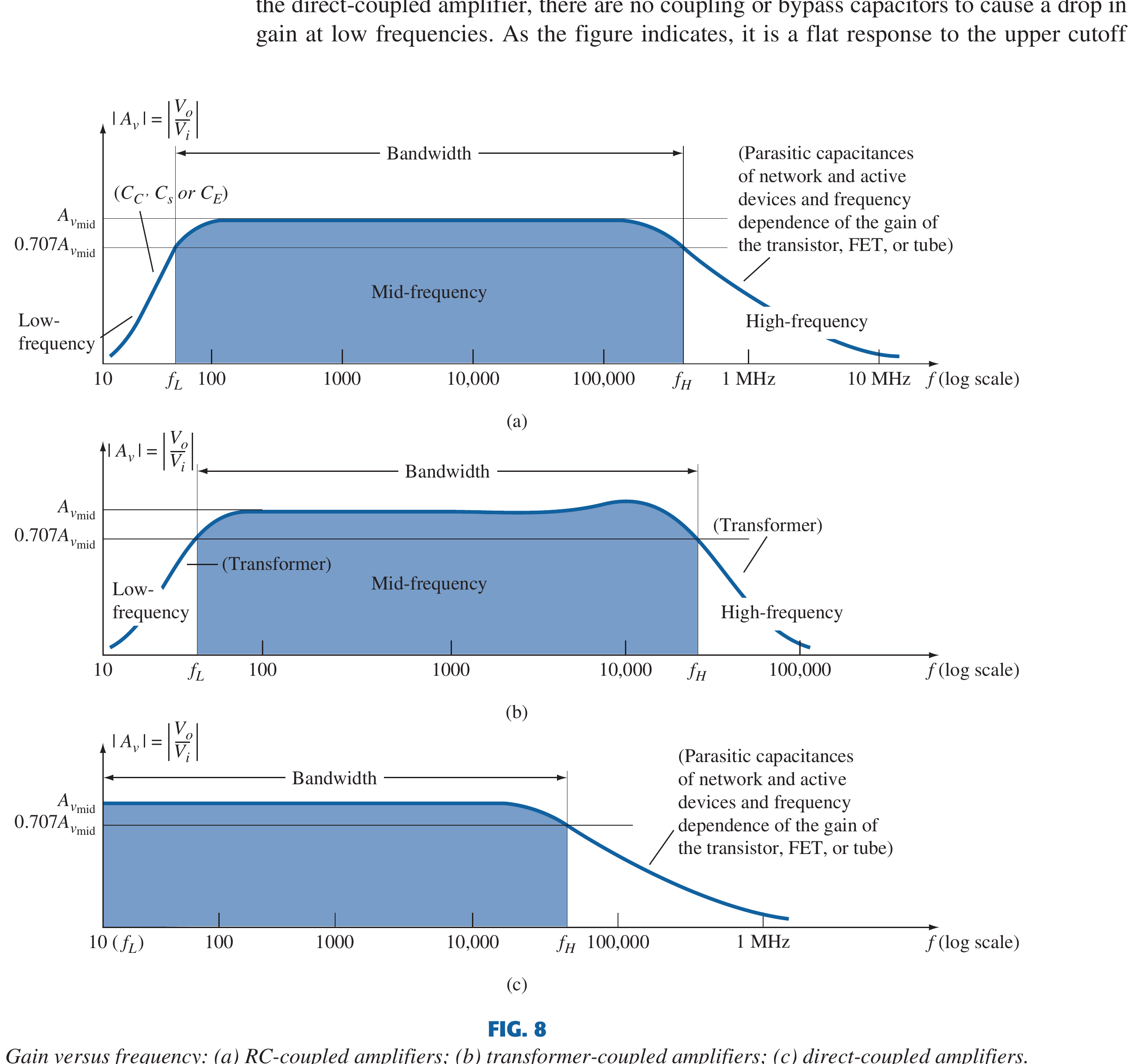
Exact magnitude and phase are
At \(\omega_c\), gain is \(3.01\) dB below \(A_0\) and phase is \(-45^\circ\).
5. Standard Responses
| Response | Passes | Key frequencies | Typical phase movement |
|---|---|---|---|
| Low-pass | Low frequencies | Upper cutoff \(f_H\) | \(0^\circ\) toward \(-90^\circ\) per pole |
| High-pass | High frequencies | Lower cutoff \(f_L\) | \(+90^\circ\) toward \(0^\circ\) per first-order section |
| Band-pass | Band between cutoffs | \(f_L,f_H\); \(BW=f_H-f_L\) | Lead below centre, zero/near-zero around centre, lag above |
| Band-stop/notch | Frequencies outside rejected band | Lower/upper stop edges; notch \(f_0\) | Rapid phase transition around rejection band |
The labels low/high-pass describe the input-to-output transfer function, not a resonator in isolation. A series or parallel resonator can realise different filtering depending on where output is measured and whether it is placed in series or shunt.
6. Loop Gain for Stability
Feedback stability is assessed from
not merely the closed-loop response. Negative feedback becomes regenerative when loop phase reaches \(-180^\circ\) modulo \(360^\circ\).
Gain Crossover and Phase Margin
At gain crossover \(\omega_{gc}\),
Phase Crossover and Gain Margin
At phase crossover \(\omega_{pc}\),
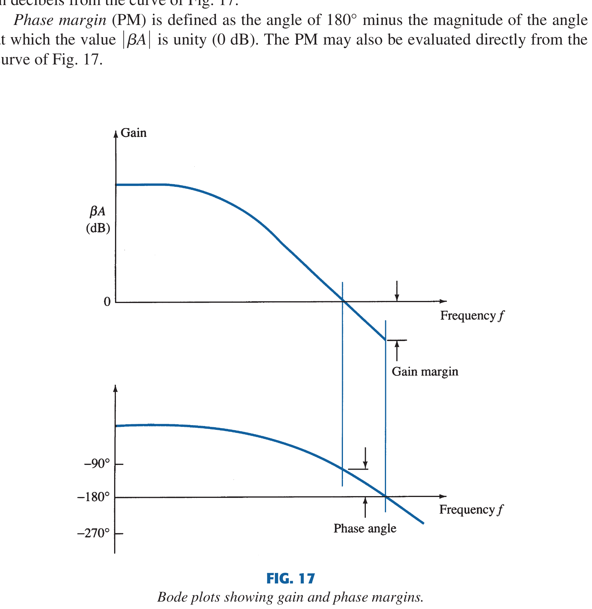
Example: if phase is \(-135^\circ\) at 0 dB crossover, \(PM=45^\circ\). If magnitude is \(-12\) dB at \(-180^\circ\) crossover, \(GM=12\) dB.
7. Interpretation and Limits
For the common case of a stable open-loop system with a conventional negative-feedback sign and a single relevant crossover:
- positive GM and PM indicate closed-loop stability;
- larger PM generally reduces ringing/overshoot but may reduce speed;
- \(PM\approx45^\circ\)–\(60^\circ\) and \(GM\gtrsim8\)–\(10\) dB are common design targets, not universal laws;
- zero/negative margin indicates marginal/unstable behaviour in that conventional case.
With right-half-plane open-loop poles, multiple 0-dB/\(-180^\circ\) crossings, delays or non-minimum-phase behaviour, a simple “positive margins” statement can be insufficient; Nyquist analysis and all crossings must be checked.
8. Frequency Compensation
- Dominant-pole compensation: introduces a low pole so loop gain crosses 0 dB before excessive phase lag accumulates; robust but slower.
- Lead compensation/zero: adds positive phase near crossover, increasing PM.
- Lag compensation: raises low-frequency loop gain relative to crossover but can slow response.
- Pole splitting/Miller compensation: widely used inside op-amps.
Compensation trades bandwidth and settling time against stability, overshoot and robustness.
9. Advantages and Applications of Bode Analysis
- quick hand construction from factored transfer functions;
- direct reading of cutoffs, bandwidth and slopes;
- combines cascaded stages by adding dB and phase;
- shows gain/phase crossover and compensation needs;
- used for feedback amplifiers, op-amps, active filters, control loops and PLLs.
Exam Traps
- Use loop gain \(A\beta\) for GM/PM, not closed-loop gain.
- PM is measured at 0 dB; GM is measured at \(-180^\circ\).
- One pole contributes an eventual \(-20\) dB/decade and up to \(-90^\circ\), not an instantaneous phase jump.
- Two poles are not automatically unstable; pole locations and crossover determine margin.
Rapid Recall
- Pole: \(-20\) dB/dec, \(-90^\circ\).
- Zero: \(+20\) dB/dec, \(+90^\circ\).
- First-order corner: \(-3.01\) dB and \(\pm45^\circ\) contribution.
- \(PM=180^\circ+\phi(\omega_{gc})\).
- \(GM_{dB}=-\lvert L\rvert_{dB}\) at \(\omega_{pc}\).
Model Answer — First-Order Amplifier Bode Plot [5 marks]
Exam-ready answer
A Bode plot gives magnitude \(20\log_{10}\lvert H(j\omega)\rvert\) and phase \(\angle H(j\omega)\) versus logarithmic frequency. For a first-order low-pass amplifier,
For \(\omega\ll\omega_c\), magnitude is approximately \(20\log_{10}A_0\) dB and phase approximately \(0^\circ\). At the corner/cutoff,
so gain is \(-3.01\) dB relative to midband and phase is \(-45^\circ\). For \(\omega\gg\omega_c\), magnitude falls at \(-20\) dB/decade (\(-6\) dB/octave) and phase tends to \(-90^\circ\).
A logarithmic axis makes decades, slopes and a wide frequency range easy to show. The plot is used to read cutoff/bandwidth and to combine pole/zero contributions for feedback stability analysis.
Practice target: 8 minutes; sketch both plots with the flat asymptote, corner point, final slope and phase limits labelled.
Model Answer — Bode Responses and Stability Margins [10 marks]
Exam-ready answer
Bode magnitude and phase plots use a logarithmic frequency axis. A simple pole contributes an eventual \(-20\) dB/decade slope and up to \(-90^\circ\) phase lag; a simple zero contributes \(+20\) dB/decade and up to \(+90^\circ\) lead. At its corner a first-order pole is \(-3.01\) dB and \(-45^\circ\).
A low-pass is flat then rolls off above \(f_H\); a high-pass rises below \(f_L\) then becomes flat; a band-pass passes \(f_L<f<f_H\) with \(BW=f_H-f_L\); a band-stop rejects a band, often with a deep notch at \(f_0\).
For feedback stability, plot loop gain \(L=A\beta\). At gain crossover \(\omega_{gc}\), \(\lvert L\rvert=1\) and
At phase crossover \(\omega_{pc}\), \(\angle L=-180^\circ\) and
If phase is \(-135^\circ\) at 0 dB, \(PM=45^\circ\); if magnitude is \(-12\) dB at \(-180^\circ\), \(GM=12\) dB. For a stable open-loop, conventional single-crossover negative-feedback system, positive margins indicate stability, while practical targets often use about \(45^\circ\)–\(60^\circ\) PM and \(8\)–\(10\) dB or more GM. Multiple crossings or open-loop right-half-plane poles require Nyquist/all-crossing analysis.
Dominant-pole compensation lowers crossover before excessive phase accumulates; lead compensation adds phase near crossover. Both trade speed/bandwidth against robustness and ringing.
Practice target: 18 minutes; sketch the four response shapes, state pole/zero rules, mark both crossovers and calculate GM/PM from one numerical reading.