Multiplexing and Traffic Engineering
Possible Exam Questions
Exam Questions and Answer Map
Tags: [PYQ paper/year] = directly observed in a past paper · [likely] = pattern-predicted variant. Marks in [ ] show the typical split.
-
Compare FDM, TDM and WDM with diagrams. [5–10] — [likely]
-
Answer plan: Define multiplexing → explain FDM principle with guard bands → explain TDM principle with time slots → explain WDM/DWDM with optical wavelengths → draw spectrum/frame diagrams → present comparison table (separation basis, medium, example, limitation).
-
Model answer: FDM, TDM and WDM Comparison
-
Explain TDM; describe the frame structure of a T1/E1 (PCM-30) system. [5–10] — [likely]
-
Answer plan: Define TDM → explain synchronous vs statistical TDM → state sampling at 8 kHz, 8 bits → derive 64 kbps per channel → describe E1 frame (32 TS, 2.048 Mbps, TS0 framing, TS16 signalling, 30 voice channels).
-
Model answer: TDM and T1/E1 PCM Frame Structure
-
Define traffic intensity (Erlang); state and apply the Erlang-B formula. [5] — [likely]
-
Answer plan: Define Erlang → state \(A = \lambda h\) → explain offered/carried/lost traffic → state Erlang B assumptions (Poisson arrival, no queue) → write formula \(B(A,m)\) → show recursive form → give a worked example.
-
Model answer: Traffic Intensity and Erlang-B Formula
-
Explain the basics of queuing theory and grade of service (GoS). [5] — [likely]
-
Answer plan: Define GoS as blocking/delay probability → introduce queue components (arrival, service, servers, discipline) → state Kendall notation → state Little’s theorem \(L = \lambda W\) → give M/M/1 key results.
- Model answer: Queuing Theory and Grade of Service
Scope of this Topic
This note covers space, time, frequency, and wavelength division multiplexing, basic multiple access ideas, Erlang traffic theory, Erlang B formula, and queuing theory used in telecom networks.
1. Multiplexing
Likely Exam Question (5 marks)
"What is multiplexing? Explain FDM and TDM with examples."
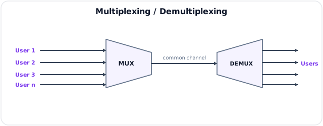
Multiplexing is the technique of combining multiple low-capacity signals into one high-capacity transmission medium. At the receiving end, demultiplexing separates the combined signal back into individual channels.
Need for Multiplexing
- Efficient use of expensive transmission media
- Increased capacity of trunks and optical fibers
- Reduction of cable, tower, repeater, and equipment cost
- Support for many users over a common system
- Better network scalability
Basic Block Diagram
2. Space Division Multiplexing (SDM)
Space Division Multiplexing separates channels by using different physical paths or spatial positions.
Examples
| Example | Explanation |
|---|---|
| Multi-pair telephone cable | Each subscriber uses a separate copper pair |
| Multi-core optical fiber | Each core carries separate traffic |
| MIMO antenna system | Different spatial paths carry different streams |
| Cellular sectorization | Different antenna sectors reuse resources spatially |
Advantages
- Simple concept
- Low signal-processing requirement
- High isolation if paths are physically separated
Limitations
- Requires more physical infrastructure
- Cable or antenna cost increases with user count
- Not efficient when transmission medium is expensive
3. Frequency Division Multiplexing (FDM)
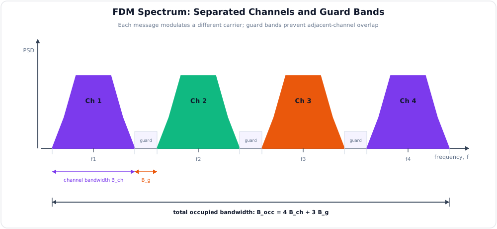
Frequency Division Multiplexing assigns each signal a separate frequency band within the total available bandwidth. All users transmit at the same time but at different frequencies.
Principle
Each baseband signal modulates a different carrier frequency. Guard bands are kept between adjacent channels to reduce interference.
Applications
| Application | Use of FDM |
|---|---|
| Radio broadcasting | Each station gets a different carrier frequency |
| Cable TV | Many TV channels share one coaxial cable |
| Analog telephone trunk | Multiple voice channels over one carrier system |
| Satellite transponder | Different carriers share transponder bandwidth |
Advantages and Disadvantages
| Advantages | Disadvantages |
|---|---|
| Continuous transmission for every user | Guard bands waste bandwidth |
| Suitable for analog signals | Requires bandpass filters and modulators |
| No time synchronization needed | Intermodulation and adjacent-channel interference possible |
4. Time Division Multiplexing (TDM)
Time Division Multiplexing allows several signals to share the same channel by assigning each signal a separate time slot.
Principle
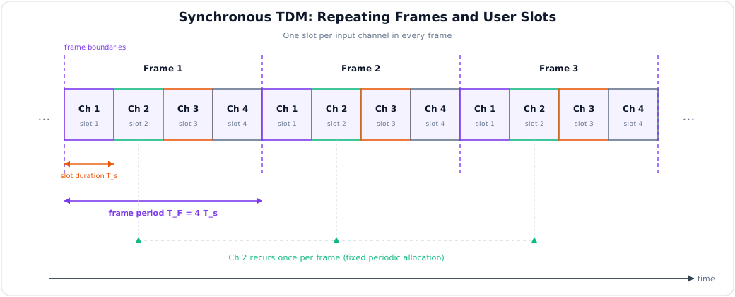
Only one user transmits in a given time slot, but the slots repeat rapidly, so communication appears continuous.
Types of TDM
| Type | Description | Example |
|---|---|---|
| Synchronous TDM | Fixed slot assigned to each channel, even if idle | PCM telephony, E1/T1 |
| Statistical TDM | Slots assigned dynamically only to active users | Packet networks |
| Asynchronous TDM | Uses address information to identify active data sources | Data multiplexers |
PCM-TDM Example
In digital telephony, voice is sampled at \(8\,\text{kHz}\) and each sample is coded into 8 bits:
An E1 system has 32 time slots:
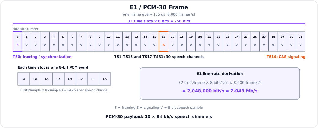
In E1, TS0 carries framing and synchronization, TS16 carries channel-associated signaling, and TS1-TS15 plus TS17-TS31 carry 30 speech channels.
Advantages and Disadvantages
| Advantages | Disadvantages |
|---|---|
| Efficient for digital signals | Requires synchronization |
| No guard bands needed | Idle slots waste capacity in synchronous TDM |
| Easy integration with digital switching | Timing jitter can affect quality |
5. Wavelength Division Multiplexing (WDM)
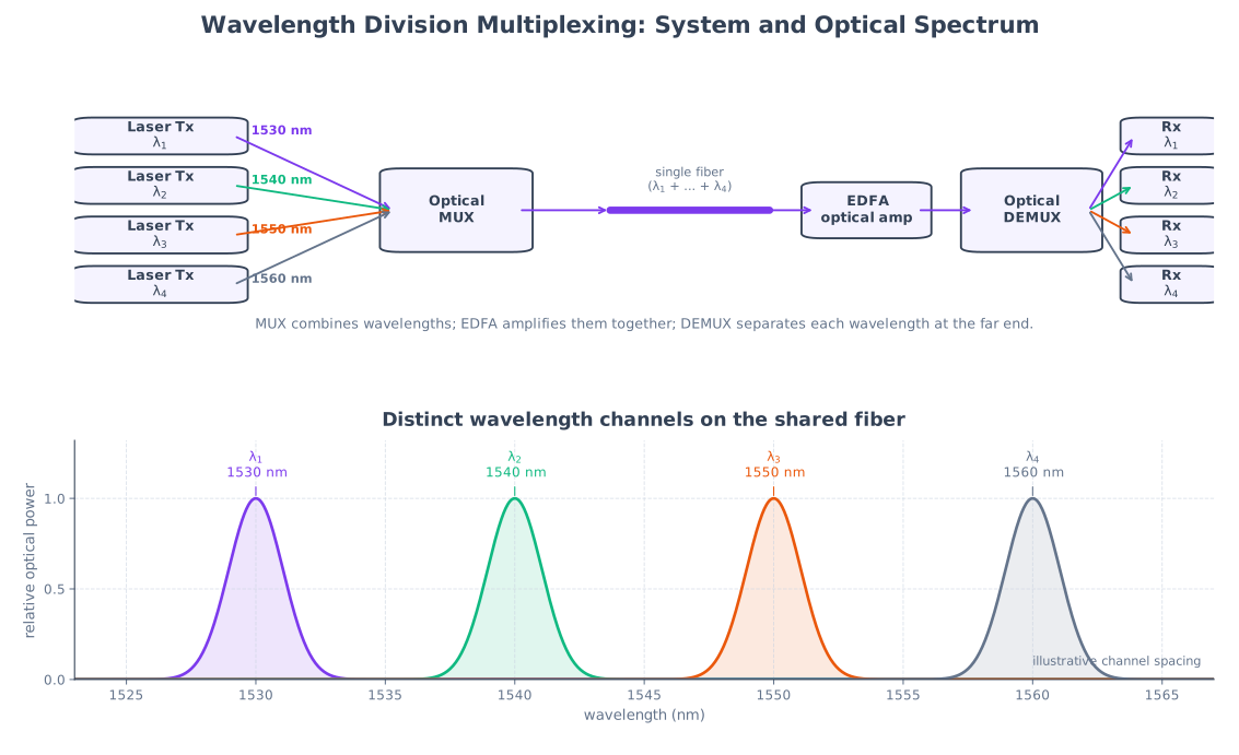
Wavelength Division Multiplexing is optical FDM. Multiple optical carriers of different wavelengths are transmitted through the same fiber.
Types of WDM
| Type | Channel Spacing | Typical Use |
|---|---|---|
| CWDM | Wide spacing, fewer wavelengths | Metro/access networks |
| DWDM | Dense spacing, many wavelengths | Long-haul and backbone networks |
Advantages
- Greatly increases fiber capacity
- Allows transparent transport of different protocols
- Supports long-distance optical backbone networks
- Existing fiber can be upgraded without laying new cable
WDM System Components
| Component | Function |
|---|---|
| Optical transmitter | Generates light at specific wavelength |
| Optical multiplexer | Combines wavelengths into one fiber |
| Optical amplifier | Amplifies optical signals without electrical conversion |
| Optical demultiplexer | Separates wavelengths at receiver |
| OADM/ROADM | Adds/drops or switches wavelengths in optical network |
6. Comparison of Multiplexing Techniques
| Technique | Separation Basis | Main Medium | Typical Example | Main Limitation |
|---|---|---|---|---|
| SDM | Physical path/space | Copper, fiber, radio space | Multi-pair cable, MIMO | More infrastructure needed |
| FDM | Frequency | Coaxial, radio, satellite | Radio, cable TV | Guard bands and filtering |
| TDM | Time slots | Digital trunks | PCM, E1/T1 | Synchronization required |
| WDM | Optical wavelength | Fiber | DWDM backbone | Optical component cost |
7. Multiplexing vs Multiple Access
Multiplexing usually describes combining multiple signals in a transmission system. Multiple access describes how multiple users share a common communication resource.
| Multiple Access | Based On | Example |
|---|---|---|
| FDMA | Frequency | 1G cellular, satellite channels |
| TDMA | Time slot | GSM |
| CDMA | Code | IS-95, CDMA2000 |
| OFDMA | Orthogonal subcarriers | LTE, WiMAX, 5G NR |
| SDMA | Space/beam | Sector antennas, MIMO beamforming |
8. Traffic Engineering
Likely Exam Question (10 marks)
"Define Erlang. Derive or explain Erlang B formula and its use in trunk dimensioning."
Teletraffic engineering is the study of traffic demand, blocking, waiting, and resource dimensioning in telecommunication networks.
Basic Terms
| Term | Meaning |
|---|---|
| Calling rate | Average number of call attempts per unit time |
| Holding time | Average duration of one call |
| Busy hour | One-hour period with maximum traffic load |
| BHCA | Busy Hour Call Attempts |
| Grade of Service (GoS) | Probability that a call is blocked or delayed beyond a limit |
| Blocking probability | Probability that a call cannot be served immediately |
Erlang
One Erlang represents continuous use of one circuit for one hour.
Traffic intensity is:
where:
- \(A\) = traffic intensity in Erlangs
- \(\lambda\) = call arrival rate in calls per unit time
- \(h\) = average holding time in the same time unit
Offered, Carried, and Lost Traffic
| Traffic Type | Meaning | Formula |
|---|---|---|
| Offered traffic | Traffic demand arriving at the system | \(A_o\) |
| Carried traffic | Traffic actually served | \(A_c = A_o(1-B)\) |
| Lost traffic | Traffic blocked by the system | \(A_l = A_oB\) |
where \(B\) is blocking probability.
9. Erlang B Formula
Erlang B is used for loss systems where blocked calls are cleared and do not wait in a queue.
Assumptions
- Call arrivals follow Poisson distribution.
- Holding time follows exponential distribution.
- There are \(m\) identical circuits or trunks.
- No waiting room exists.
- If all trunks are busy, the call is blocked and cleared.
Formula
For offered traffic \(A\) and number of trunks \(m\):
Recursive form used for calculation:
Use of Erlang B
- Determine number of trunks for a target GoS
- Estimate call blocking probability
- Dimension PSTN, mobile, and inter-exchange trunk groups
- Plan expansion of exchange capacity
10. Queuing Theory
Likely Exam Question (5 marks)
"State Little's theorem and explain its significance in communication networks."
Queuing theory analyzes systems where users, calls, or packets wait for service. It is important in packet buffers, routers, call centers, switching systems, and access networks.
Queue Components
| Component | Meaning |
|---|---|
| Arrival process | Pattern of customer/packet arrivals |
| Service process | Time required to serve one customer/packet |
| Number of servers | Number of parallel service channels |
| Queue discipline | Rule for service order, e.g. FIFO, priority, round-robin |
| Queue capacity | Maximum number of waiting customers/packets |
Kendall Notation
Queue models are written as:
where:
| Symbol | Meaning |
|---|---|
| \(A\) | Arrival distribution |
| \(S\) | Service-time distribution |
| \(c\) | Number of servers |
| \(K\) | System capacity |
| \(N\) | Population size |
| \(D\) | Queue discipline |
Common notation: M/M/1 means Markovian arrival, Markovian service, and one server.
Little's Theorem
For a stable queuing system:
where:
- \(L\) = average number of items in system
- \(\lambda\) = average arrival rate
- \(W\) = average time spent in system
Similarly, for the waiting queue only:
Little's theorem is general and does not depend on the arrival or service distribution, as long as the system is stable.
11. M/M/1 Queue
For a single-server queue with Poisson arrival rate \(\lambda\) and exponential service rate \(\mu\):
Utilization
For stable operation:
Main Results
| Quantity | Formula |
|---|---|
| Probability of zero items | \(P_0 = 1-\rho\) |
| Average number in system | \(L = \dfrac{\rho}{1-\rho}\) |
| Average number in queue | \(L_q = \dfrac{\rho^2}{1-\rho}\) |
| Average time in system | \(W = \dfrac{1}{\mu-\lambda}\) |
| Average waiting time in queue | \(W_q = \dfrac{\lambda}{\mu(\mu-\lambda)}\) |
As \(\rho\) approaches 1, delay increases sharply. Therefore a telecom system should not be planned with utilization too close to 100%.
12. Erlang B vs Queuing Model
| Feature | Erlang B | Queuing Model |
|---|---|---|
| System type | Loss system | Waiting system |
| Blocked user | Cleared immediately | Waits in queue |
| Main metric | Blocking probability | Waiting time and queue length |
| Example | Trunk group without waiting | Router buffer, call center |
| Typical formula | Erlang B | Little's law, M/M/1, M/M/c |
13. Solved Examples
Example 1 - Traffic Intensity
Q. A subscriber makes 4 calls in the busy hour. Average call duration is 3 minutes. Find traffic offered by the subscriber.
Solution:
Total call time in one hour:
Traffic in Erlang:
Example 2 - Erlang B
Q. Find blocking probability for \(A = 2\) Erlangs and \(m = 4\) trunks.
Solution:
Blocking probability is approximately 9.52%.
Example 3 - M/M/1 Queue
Q. Packets arrive at a router at \(80\) packets/s. The router can serve \(100\) packets/s. Find utilization, average number in the system, and average delay.
Solution:
The router utilization is 80%, average number of packets in the system is 4, and average delay is 50 ms.
Key Exam Points - Multiplexing and Traffic
- FDM separates users by frequency; TDM separates users by time; WDM separates optical channels by wavelength; SDM separates users by physical/spatial path.
- One Erlang means one circuit occupied continuously for one hour.
- Traffic intensity: \(A = \lambda h\).
- Erlang B gives blocking probability in a loss system with no waiting queue.
- Little's theorem: \(L = \lambda W\).
- For M/M/1, stability requires \(\lambda < \mu\) or \(\rho < 1\).
Model Answer - FDM, TDM and WDM Comparison [5-10 marks]
5-mark answer and 10-mark extension
For 5 marks - FDM, TDM and WDM principles
Multiplexing combines several independent tributaries for transmission over one higher-capacity link; a demultiplexer separates them at the destination. FDM translates each input onto a different carrier so all channels occupy non-overlapping frequency bands simultaneously. Bandpass filters and guard bands limit adjacent-channel interference. It suits radio, cable TV, satellite transponders, and analog carrier telephony.
TDM gives each input the full link bandwidth for a recurring time slot. Synchronous TDM reserves fixed slots, whereas statistical TDM labels and assigns slots only to active inputs. It suits PCM trunks such as E1/T1 and requires common clock and frame synchronization.
WDM is optical frequency multiplexing: lasers at distinct wavelengths \(\lambda_1,\lambda_2,\ldots\) are optically combined onto one fiber and separated by filters at the receiver. CWDM uses wider spacing and fewer channels; DWDM uses dense spacing for high-capacity long-haul systems.
Add for a 10-mark multiplexing comparison
The operating paths differ. In FDM, each source modulates a carrier, a summer forms the composite spectrum, and the receiver selects, demodulates, and low-pass-filters each band. If channel bandwidth is \(B_i\) and guard interval is \(G_i\), the link requires approximately \(B_T\ge\sum B_i+\sum G_i\). Nonlinear devices can create intermodulation products, so linear amplification and sharp filters matter.
In synchronous TDM, a commutator reads one sample or word from each tributary, adds framing/signaling where required, and transmits a serial frame; the receiving clock and frame detector drive the inverse commutator. For \(N\) tributaries each contributing \(b\) bits at \(f_s\) samples/s, ignoring overhead, \(R_b=Nbf_s\). Slots assigned to idle sources waste capacity, while statistical TDM improves utilization at the cost of addresses, buffering, and variable delay.
In WDM, optical sources must remain within wavelength tolerances; a MUX, fiber, EDFA/repeater, optional OADM/ROADM, and DEMUX form the path. Chromatic dispersion, nonlinear fiber effects, amplifier noise, and component cost limit reach/channel count, but each wavelength can transparently carry Ethernet, SDH, or another format.
| Feature | FDM | TDM | WDM |
|---|---|---|---|
| Separation | Frequency bands | Time slots | Optical wavelengths |
| Simultaneous inputs | Yes | No, interleaved | Yes |
| Main medium | Radio/coax/copper | Digital copper, radio, fiber | Optical fiber |
| Overhead/isolation | Guard bands and filters | Framing, clock, buffers | Optical spacing and filters |
| Example | FM broadcast/CATV | PCM E1 | DWDM backbone |
Thus FDM is natural for continuous analog/RF channels, TDM for synchronized digital streams, and WDM for multiplying fiber capacity. Actual channel spacings, wavelength grids, and payload efficiency are system- and standard-dependent.
Practice target: 9 minutes for the 5-mark principles or 18 minutes for all paths, equations, diagrams, and the comparison table.
Model Answer - TDM and T1/E1 PCM Frame Structure [5-10 marks]
5-mark answer and 10-mark extension
For 5 marks - TDM and E1 core
Time-division multiplexing (TDM) shares one digital link by interleaving tributary words in time. A transmitter samples each source, inserts its bits into an assigned slot, and adds framing/signaling; a synchronized receiver identifies frame boundaries and routes each slot to the corresponding output. Synchronous TDM gives every source a fixed slot even when idle. Statistical TDM allocates labeled slots to active sources, increasing efficiency but introducing addressing, buffering, and variable delay.
Telephone speech is nominally low-pass limited to about \(3.4\,\text{kHz}\) and sampled at \(f_s=8\,\text{kHz}\). With 8-bit PCM,
European E1/PCM-30 interleaves 32 time slots, each 8 bits, once every \(125\,\mu\text{s}\); 30 slots can carry speech, TS0 carries framing/alarms, and TS16 is conventionally allocated to channel-associated signaling.
Add for a 10-mark E1/T1 extension
One E1 frame therefore contains
and its gross line rate is
TS1-TS15 and TS17-TS31 provide the 30 nominal \(64\,\text{kbit/s}\) bearer channels, totaling \(1.920\,\text{Mbit/s}\). TS0 carries frame alignment and service information. In the common PCM-30 channel-associated-signaling convention, TS16 carries signaling arranged over a 16-frame multiframe; other signaling arrangements, including common-channel signaling, are network-dependent, so “TS16 always carries CAS” is not universal. E1 line coding and detailed CRC/multiframe use also depend on the deployed recommendation.
The North American/Japanese T1/DS1 convention differs: each \(125\,\mu\text{s}\) frame has 24 eight-bit channel words plus one framing bit, hence \(24\times8+1=193\) bits and
Signaling may use robbed bits under traditional channel-associated arrangements. Therefore E1 is not merely T1 with a different name: slot count, framing, signaling, line rate, and regional standards differ.
Operationally, the PCM encoder anti-alias-filters, samples, compands and encodes each analog channel; the multiplexer reads one octet from each tributary, emits TS0 through TS31, and repeats at \(8\,\text{kHz}\). The receiver recovers clock, detects framing, demultiplexes slots, decodes PCM, and reconstructs speech. TDM provides deterministic channel rate and straightforward digital switching, but fixed idle slots consume capacity and slips/jitter or loss of frame alignment impair many channels together. E1 is used between exchanges, PBXs, radio base stations, and legacy access multiplexers.
Practice target: 9 minutes for the E1 core or 18 minutes for E1/T1 arithmetic, frame diagram, operation, and signaling caveat.
Model Answer - Traffic Intensity and Erlang-B Formula [5 marks]
Exam-ready answer
Traffic intensity is the average simultaneous occupancy offered to a telecom resource. If calls arrive at mean rate \(\lambda\) calls per unit time and have mean holding time \(h\) in the same unit,
One Erlang means one circuit occupied continuously, for example one 60-minute call or thirty 2-minute calls during an hour. Offered traffic \(A_o\) is attempted demand; with blocking probability \(B\), carried traffic is approximately \(A_c=A_o(1-B)\) and lost traffic \(A_l=A_oB\). Grade of service (GoS) for a loss trunk group is commonly the busy-hour probability that an offered call is blocked.
For \(m\) identical circuits, Poisson arrivals, independent exponential holding times, full availability, and blocked calls cleared without a queue, Erlang-B gives
A numerically convenient recursion is
Example: for \(A=2\) Erlangs and \(m=4\) trunks,
About 9.52% of attempts are blocked, so this group fails a target GoS of 1% and needs more circuits or less offered load. Engineers invert the table/recursion to dimension PSTN or mobile trunk groups. Erlang-B is not a waiting model and does not predict queue delay; retrials, non-Poisson bursts, reserved circuits, and finite sources require another model or simulation.
Practice target: 8 minutes; define one Erlang, state all loss-system assumptions, write direct and recursive forms, and interpret the worked probability.
Model Answer - Queuing Theory and Grade of Service [5 marks]
Exam-ready answer
Queuing theory models calls, packets, or users that arrive, wait if service is unavailable, receive service, and depart. A queue is specified by its arrival process, service-time distribution, number of parallel servers, system capacity, calling population, and discipline such as FIFO or priority. Kendall notation \(A/S/c/K/N/D\) records these features; M/M/1 means Poisson (Markovian) arrivals, exponential service, one server, conventionally infinite capacity/population and FIFO when omitted.
Grade of service (GoS) quantifies customer impairment. In a loss system it is commonly blocking probability; in a delay system it may be mean delay or \(P\{W_q>t\}\). It must therefore be stated with its metric and busy-hour condition. For any stable system with effective arrival rate \(\lambda\),
where \(L,W\) refer to the whole system and \(L_q,W_q\) to only the waiting line. Little's law is distribution-independent but requires consistent averages and a stable observation period.
For an M/M/1 server of rate \(\mu\),
Example: a router with \(\lambda=80\) packets/s and \(\mu=100\) packets/s has \(\rho=0.8\), \(L=4\) packets and \(W=0.05\) s; \(L=\lambda W=4\) verifies Little's law. As utilization approaches unity, delay rises sharply, so capacity needs headroom. Unlike Erlang-B, which clears a blocked call and measures loss, a router buffer admits waiting and trades lower loss for delay; finite buffers, bursty traffic, priorities, and non-exponential service require models beyond M/M/1.
Practice target: 8 minutes; define the queue and GoS metric, write Little's law and M/M/1 stability/results, then interpret one numerical example.