Feedback Amplifiers¶

Possible Exam Questions¶

Exam Questions and Answer Map

Define negative feedback, derive closed-loop gain and discuss its effects on amplifier performance. [10] — [likely]
Answer plan: Draw summing loop → derive \(A_f=A/(1+A\beta)\) → define loop gain and sensitivity → discuss gain, bandwidth, distortion, internal noise, stability and impedance with assumptions.
Model answer: Negative-Feedback Gain and Performance Effects
Explain the four feedback topologies and their impedance effects. [5] — [likely]
Answer plan: Classify by input mixing and output sampling → use series/shunt rules → name stabilised gain quantity for each topology.
Model answer: Four Feedback Topologies

1. Feedback Concept¶

Feedback returns a fraction of amplifier output to its input.

Negative (degenerative) feedback: returned signal opposes the source, reducing error and closed-loop gain. It is used to improve controlled amplifier behaviour.
Positive (regenerative) feedback: returned signal reinforces the source. It is used for oscillation, hysteresis and switching; excessive positive feedback makes a linear amplifier unstable.

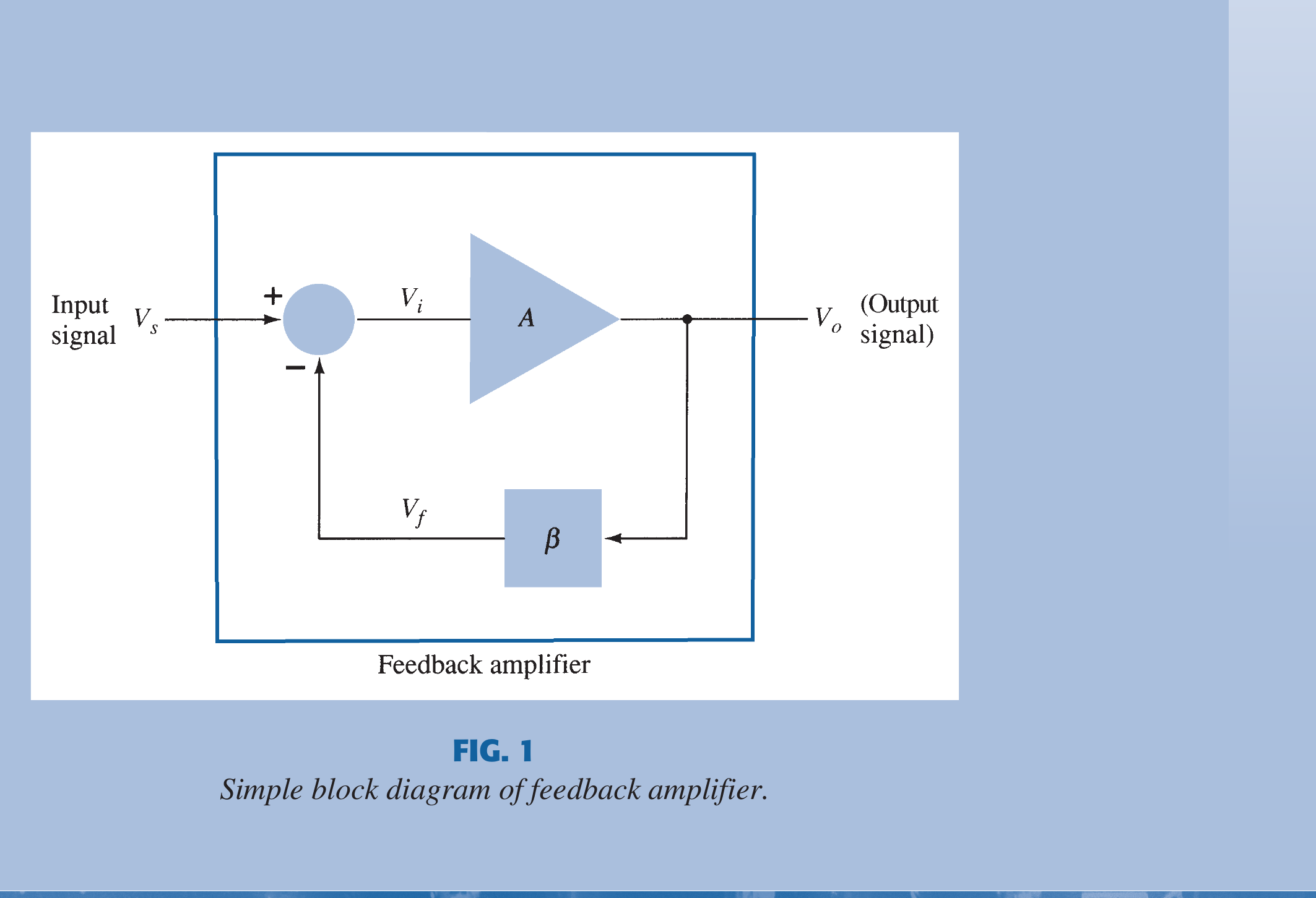
Fig: Textbook negative-feedback amplifier block diagram

2. Closed-Loop Gain Derivation¶

Let source be \(x_s\), error/input to the forward amplifier be \(x_e\), output be \(x_o\), forward gain \(A\) and feedback factor \(\beta\):

\[ x_e=x_s-\beta x_o, \qquad x_o=Ax_e. \]

Substitution gives

\[ x_o=A(x_s-\beta x_o), \]

\[ x_o(1+A\beta)=Ax_s, \]

\[ \boxed{A_f=\frac{x_o}{x_s}=\frac{A}{1+A\beta}}. \]

The complex, frequency-dependent quantity

\[ \boxed{L(s)=A(s)\beta(s)} \]

is loop gain. \(1+L\) is the return difference. If \(\lvert L\rvert\gg1\) while phase remains genuinely negative feedback,

\[ A_f\approx\frac{1}{\beta}. \]

For positive feedback under the same sign convention, \(A_f=A/(1-A\beta)\).

3. Gain Desensitivity¶

For scalar \(A,\beta\),

\[ \boxed{\frac{dA_f/A_f}{dA/A}=\frac{1}{1+A\beta}}. \]

Thus high negative loop gain makes closed-loop gain less sensitive to transistor gain, temperature and supply variation. This is a local/in-band statement; \(L\) falls and rotates in phase with frequency.

4. Effects of Negative Feedback¶

Gain¶

Gain decreases by the factor \(1+L\) but becomes more predictable. This is a deliberate exchange of excess open-loop gain for accuracy.

Bandwidth¶

For a stable single-dominant-pole amplifier with approximately frequency-independent \(\beta\) in the band,

\[ f_{Hf}\approx f_H(1+L_0), \qquad f_{Lf}\approx\frac{f_L}{1+L_0}. \]

Closed-loop bandwidth therefore increases and gain-bandwidth product is approximately conserved in this model. These are not universal identities for arbitrary multipole amplifiers.

Distortion¶

Nonlinear distortion generated inside the forward path and enclosed by the loop is reduced approximately by \(1+\lvert L\rvert\) while sufficient loop gain remains. Output-stage dead zones, slew limits and clipping cannot be assumed to disappear.

Noise¶

Noise generated inside the enclosed forward path can be reduced at output relative to signal by feedback. Input/source noise and feedback-network thermal noise are not automatically reduced; feedback may even increase required noise bandwidth.

Stability and Transient Response¶

Negative feedback improves parameter stability, but frequency-dependent phase lag can turn the returned signal into effective positive feedback. Poor phase margin causes ringing or oscillation. Feedback therefore improves gain stability while requiring a separate loop stability check.

Input and Output Impedance¶

Impedance changes depend on how feedback is mixed and sampled, not merely on the word “negative.” Series input mixing raises \(Z_{in}\); shunt input mixing lowers it. Voltage sampling lowers \(Z_{out}\); current sampling raises it.

5. Four Feedback Topologies¶

A feedback amplifier is classified by what it samples at the output (a voltage or a current) and how it mixes the fed-back signal at the input (in series or in shunt). The two output choices times the two input choices give four topologies, and each maps one-to-one onto one of the four amplifier types.

Amplifier type (out–in)	Gain	Feedback name (sample–mix)	Connection (in–out)	Output sampled	Input mixing	Typical effect
Voltage–voltage (voltage amplifier)	\(A_v=\dfrac{V_o}{V_i}\)	Voltage-series	Series–shunt	Voltage (shunt)	Series	\(R_{in}\uparrow,\ R_{out}\downarrow\)
Voltage–current (transresistance)	\(R_m=\dfrac{V_o}{I_i}\)	Voltage-shunt	Shunt–shunt	Voltage (shunt)	Shunt	\(R_{in}\downarrow,\ R_{out}\downarrow\)
Current–voltage (transconductance)	\(G_m=\dfrac{I_o}{V_i}\)	Current-series	Series–series	Current (series)	Series	\(R_{in}\uparrow,\ R_{out}\uparrow\)
Current–current (current amplifier)	\(A_i=\dfrac{I_o}{I_i}\)	Current-shunt	Shunt–series	Current (series)	Shunt	\(R_{in}\downarrow,\ R_{out}\uparrow\)

With \(D=1+A\beta\) in the useful negative-feedback band, series input mixing scales \(Z_{in}\) by \(\times D\) and shunt mixing by \(\div D\); voltage sampling scales \(Z_{out}\) by \(\div D\) and current sampling by \(\times D\).

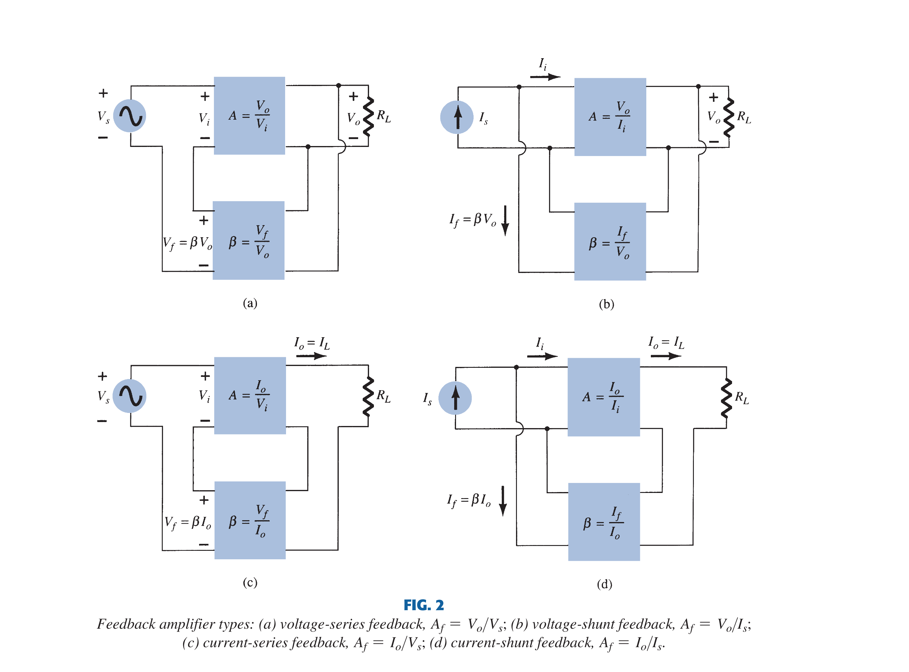
Fig: Textbook two-port constructions for voltage-series, voltage-shunt, current-series and current-shunt feedback

Book-grounded topology decoder

Determine the topology in two questions: What is sampled at the output? (voltage across the port or current through it) and How is feedback mixed at the input? (series voltage or shunt current). This is safer than memorizing four names in isolation.

Source figure: Boylestad/Nashelsky, Electronic Devices and Circuit Theory (11th ed.), PDF p. 781.

Two-Port Small-Signal Models¶

Each topology is drawn as a small-signal two-port: the driving source (a Thévenin \(V_s\)–\(R_s\) pair for series mixing or a Norton \(I_s\parallel R_s\) pair for shunt mixing), the amplifier (\(R_i\) at the input and a dependent source with output resistance \(R_o\)), the load \(R_L\), and the feedback network that samples the output and returns its signal to the input.

(a) Voltage-series (series–shunt) — voltage amplifier; the feedback voltage \(\beta V_o\) is mixed in series at the input and the output voltage is sampled in shunt.

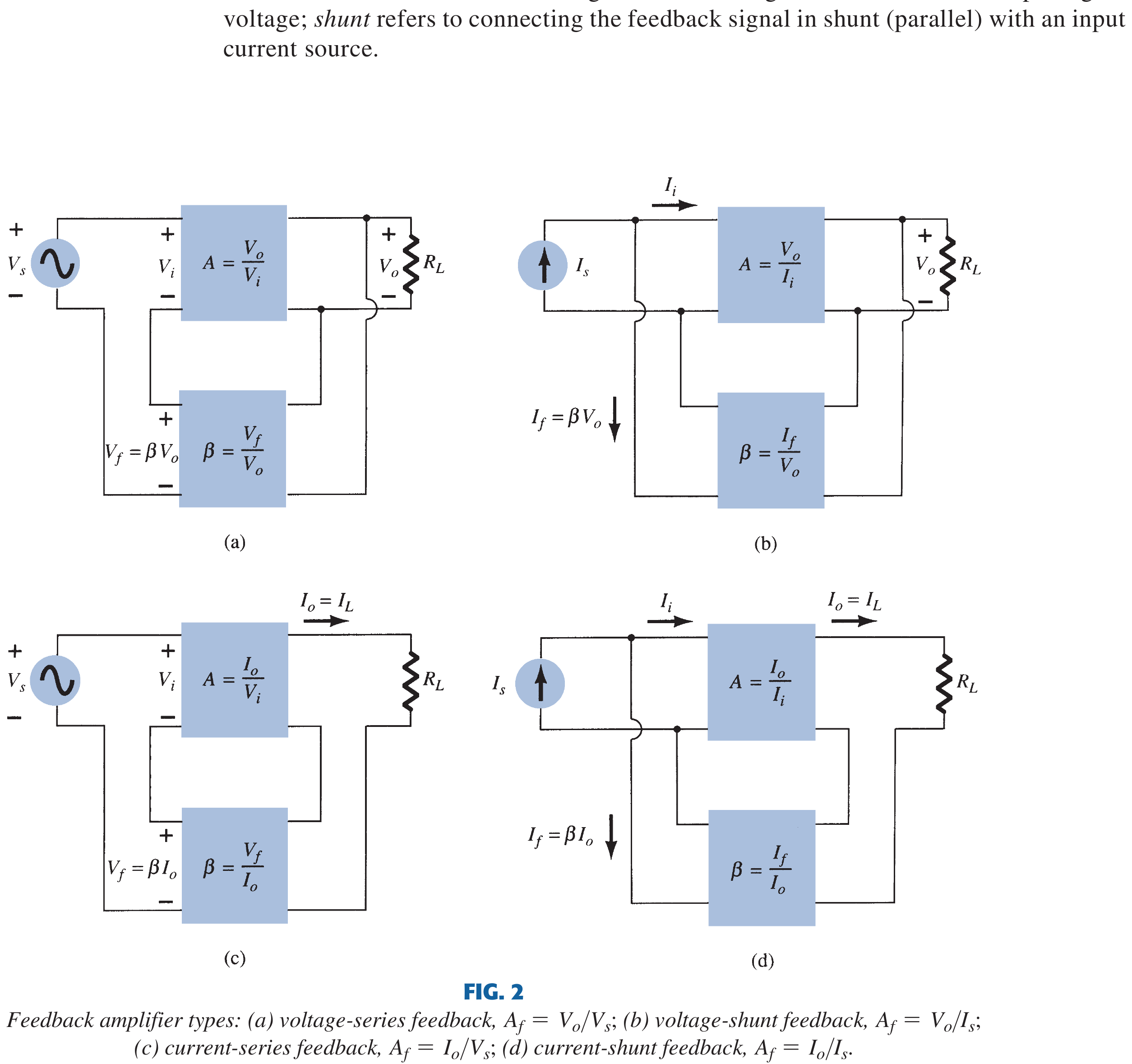
Fig: Textbook voltage-series feedback connection

(b) Current-series (series–series) — transconductance amplifier; the feedback voltage \(\beta I_o\) is mixed in series at the input and the output current is sampled in series.

Fig: Textbook current-series feedback connection

(c) Current-shunt (shunt–series) — current amplifier; the feedback current \(\beta I_o\) is mixed in shunt at the input and the output current is sampled in series.

Fig: Textbook current-shunt feedback connection

(d) Voltage-shunt (shunt–shunt) — transresistance amplifier; the feedback current \(\beta V_o\) is mixed in shunt at the input and the output voltage is sampled in shunt.

Fig: Textbook voltage-shunt feedback connection

Memory Rule¶

Series at input obstructs source current → \(Z_{in}\) increases.
Shunt at input provides another current path → \(Z_{in}\) decreases.
Voltage sampling seeks a stiff voltage source → \(Z_{out}\) decreases.
Current sampling seeks a stiff current source → \(Z_{out}\) increases.

6. Advantages, Disadvantages and Applications¶

Advantages¶

stable, accurately set closed-loop gain;
wider bandwidth in common dominant-pole designs;
lower enclosed distortion and some internally generated noise;
useful control of input/output impedances;
improved linearity and tolerance to device variation.

Disadvantages¶

reduced gain;
risk of high-frequency ringing/oscillation;
compensation may reduce speed;
feedback components add noise, tolerance and loading;
large-signal limits and out-of-loop errors remain.

Applications¶

Op-amp circuits, audio amplifiers, instrumentation amplifiers, automatic gain/control loops, voltage/current regulators, active filters and communication receiver/transmitter stages.

Exam Traps

\(A_f=A/(1+A\beta)\) assumes the drawn negative-feedback sign convention.
Noise/distortion reduction applies to errors generated inside the effective loop.
“Bandwidth multiplies by \(1+A\beta\)” is a dominant-pole approximation.
Gain stability and loop stability are different ideas.

Rapid Recall¶

Error: \(x_e=x_s-\beta x_o\).
Loop gain: \(L=A\beta\).
Closed-loop gain: \(A_f=A/(1+L)\).
Series input → \(Z_{in}\) up; shunt input → down.
Voltage sampling → \(Z_{out}\) down; current sampling → up.

Model Answer — Negative-Feedback Gain and Performance Effects [10 marks]¶

Exam-ready answer

Negative feedback returns a fraction \(\beta\) of output in opposition to source. With error \(x_e=x_s-\beta x_o\) and output \(x_o=Ax_e\),

\[ x_o=A(x_s-\beta x_o) \]

gives

\[ \boxed{A_f=\frac{x_o}{x_s}=\frac{A}{1+A\beta}}. \]

\(L=A\beta\) is loop gain and \(1+L\) the return difference. For \(\lvert L\rvert\gg1\) with adequate phase margin, \(A_f\approx1/\beta\). Gain sensitivity is

\[ \frac{dA_f/A_f}{dA/A}=\frac1{1+A\beta}, \]

so transistor/supply/temperature gain changes have much smaller closed-loop effect.

Negative feedback reduces gain but, for a stable dominant-pole amplifier with nearly constant \(\beta\), increases upper cutoff and decreases lower cutoff by roughly \(1+L_0\), widening bandwidth while approximately preserving gain-bandwidth product. Nonlinear distortion and noise generated inside the enclosed forward path are reduced approximately by loop gain where it remains large; source noise, feedback-network noise, clipping, slew limiting and out-of-loop errors are not automatically removed.

Impedance depends on topology: series input mixing raises \(Z_{in}\) and shunt mixing lowers it; voltage sampling lowers \(Z_{out}\) and current sampling raises it. Feedback improves gain accuracy but phase lag can make it regenerative at high frequency, so gain and phase margins must be checked.

Advantages are predictable gain, wider useful band, improved linearity and controllable impedances. Disadvantages are lost gain, extra components/noise and possible ringing or oscillation. Applications include op-amps, audio, instrumentation, active filters and regulators.

Practice target: 18 minutes; derive the denominator from the summing equation, state five qualified effects, reproduce the impedance rules and end with the stability trade-off.

Model Answer — Four Feedback Topologies [5 marks]¶

Exam-ready answer

Feedback topology is named by input mixing (series or shunt) and output sampling (voltage/shunt or current/series).

Fig: Textbook four feedback-amplifier connection types

Topology	Stabilised gain	Input impedance	Output impedance
Voltage-series	Voltage gain	Increases	Decreases
Voltage-shunt	Transresistance	Decreases	Decreases
Current-series	Transconductance	Increases	Increases
Current-shunt	Current gain	Decreases	Increases

If \(D=1+A\beta\), series mixing multiplies \(Z_{in}\) by \(D\) and shunt mixing divides it by \(D\). Voltage sampling divides \(Z_{out}\) by \(D\), producing a stiffer voltage source; current sampling multiplies \(Z_{out}\) by \(D\), producing a stiffer current source.

The memory rule is therefore: series input up, shunt input down; voltage output down, current output up. These changes hold in the frequency range where the feedback remains negative and the corresponding loop gain is effective.

Practice target: 8 minutes; reproduce the four-row table from the two input and two output rules without memorising four isolated cases.