Magnetostatics
Possible Exam Questions
Exam Questions and Answer Map
Questions labelled [PYQ paper/year] are observed past questions; those labelled [likely] are pattern-based predictions. For each one, rehearse the answer plan closed-book, then use the links to verify the full answer in this chapter.
- State Biot-Savart's law and Ampere's circuital law; give one application of each. [5] — [likely]
- Answer plan: State Biot-Savart law (integral form for \(d\vec H\)) → state Ampere's circuital law \(\oint\vec H\cdot d\vec l = I_{\text{enc}}\) → give one application of each (e.g., field of finite wire; solenoid field).
- Model answer: Biot-Savart and Ampere laws with applications
- Use Ampere's law to find H for an infinite straight conductor, a solenoid and a toroid. [5] — [likely]
- Answer plan: Choose Amperian path for each → apply symmetry → evaluate closed-line integral → solve for \(H\) → state final expressions.
- Model answer: Ampere-law fields of a wire, solenoid, and toroid
- Define curl and state its physical significance (∇×H = J). [5] — [likely]
- Answer plan: Define curl as circulation per unit area → write Cartesian determinant form → state \(\nabla\times\vec H = \vec J\) → explain physical meaning (current density equals curl of \(H\)) → mention Stokes' theorem link.
- Model answer: Curl and the point form of Ampere's law
- Differentiate between scalar and vector magnetic potential. [5] — [PYQ 2081]
- Answer plan: Define scalar magnetic potential \(V_m\) where \(\vec H = -\nabla V_m\) (valid only in current-free region) → define vector potential \(\vec A\) where \(\vec B = \nabla\times\vec A\) → compare applicability, governing equations, and uniqueness.
- Model answer: Scalar and vector magnetic potentials
- Derive the expression for magnetic boundary conditions (normal B, tangential H). [5] — [PYQ 2081]
- Answer plan: Apply \(\nabla\cdot\vec B = 0\) across pillbox → derive \(B_{1n}=B_{2n}\) → apply Ampere's law along rectangular loop → derive \(\hat a_n\times(\vec H_2 - \vec H_1)=\vec K_s\) → state simplified forms for no surface current.
- Model answer: Magnetic boundary conditions
Syllabus Focus
- Biot-Savart's law
- Ampere's circuital law
- Curl
1. Introduction to Magnetostatics
Likely Exam Question (5 marks)
"Define magnetostatics. Compare electrostatic and magnetostatic fields."
Magnetostatics deals with magnetic fields produced by steady currents. A current is steady when its magnitude and distribution do not vary with time.
In electrostatics, stationary charges produce electric fields. In magnetostatics, moving charges or steady currents produce magnetic fields.
| Electrostatics | Magnetostatics |
|---|---|
| Source is electric charge \(Q\) or \(\rho_v\) | Source is current \(I\) or current density \(\vec J\) |
| Field quantity is \(\vec E\) | Field quantity is \(\vec H\) or \(\vec B\) |
| Basic law is Coulomb's law | Basic law is Biot-Savart's law |
| Integral law is Gauss' law | Integral law is Ampere's circuital law |
| \(\nabla \cdot \vec D = \rho_v\) | \(\nabla \times \vec H = \vec J\) |
| Electric field lines start/end on charges | Magnetic flux lines are closed loops |
Magnetic Field Quantities
| Quantity | Symbol | Unit |
|---|---|---|
| Magnetic field intensity | \(\vec H\) | A/m |
| Magnetic flux density | \(\vec B\) | tesla (T) or Wb/m\(^2\) |
| Magnetic flux | \(\Phi\) | weber (Wb) |
| Permeability | \(\mu\) | H/m |
| Free-space permeability | \(\mu_0\) | \(4\pi \times 10^{-7}\,\text{H/m}\) |
For a linear, isotropic medium:
where \(\mu_r\) is relative permeability.
Current and Current Density
Current is the rate of flow of charge:
Volume current density:
Unit: A/m\(^2\)
For a conductor with conductivity \(\sigma\) under electric field \(\vec E\):
This is the point form of Ohm's law.
Common current densities:
| Type | Symbol | Unit | Current Element |
|---|---|---|---|
| Line current | \(I\) | A | \(I\,d\vec l\) |
| Surface current density | \(\vec K\) | A/m | \(\vec K\,dS\) |
| Volume current density | \(\vec J\) | A/m\(^2\) | \(\vec J\,dv\) |
2. Magnetic Force and Lorentz Force
Likely Exam Question (5 marks)
"State the force on a moving charge and current-carrying conductor in a magnetic field."
Force on a Moving Charge
A charge \(Q\) moving with velocity \(\vec u\) in a magnetic field \(\vec B\) experiences force:
Magnitude:
where \(\theta\) is the angle between \(\vec u\) and \(\vec B\).
Important points:
- Magnetic force is perpendicular to both velocity and magnetic field.
- Magnetic force does no work because it is perpendicular to motion.
- Maximum force occurs when \(\theta = 90^\circ\).
- Zero force occurs when the charge moves parallel to \(\vec B\).
Lorentz Force
If both electric and magnetic fields are present:
Force on a Current-Carrying Conductor
For a conductor carrying current \(I\) in magnetic field \(\vec B\):
For a straight conductor of length \(L\) in uniform magnetic field:
Magnitude:
Torque on a Current Loop
For a current loop with \(N\) turns, area \(A\), and current \(I\):
where magnetic dipole moment is:
Magnitude:
This is the operating principle of moving-coil instruments and DC motors.
3. Biot-Savart's Law
Likely Exam Question (10 marks)
"State Biot-Savart's law. Derive the magnetic field due to a long straight current-carrying conductor."
Statement
Biot-Savart's law gives the magnetic field intensity produced at a point by a differential current element.
For a line current element \(I\,d\vec l\):
where:
- \(I\) is current in amperes.
- \(d\vec l\) is the differential length element in the direction of current.
- \(R\) is the distance from the current element to the observation point.
- \(\hat a_R\) is the unit vector from the current element to the observation point.
Magnetic flux density form:
Integral Forms
For a line current:
For a surface current:
For a volume current:
Direction of Magnetic Field
The direction is found using the right-hand rule:
- Thumb points in the direction of current.
- Curled fingers show direction of magnetic field around the conductor.
4. Standard Results from Biot-Savart's Law
4.1 Infinite Straight Current-Carrying Conductor
For an infinitely long wire carrying current \(I\), the magnetic field at radial distance \(\rho\) is:
The field circles the wire and decreases as \(1/\rho\).
4.2 Finite Straight Conductor
For a finite straight conductor, if the observation point is at perpendicular distance \(\rho\) and the conductor subtends angles \(\alpha_1\) and \(\alpha_2\) at that point:
For symmetric angles \(\alpha_1 = -\alpha\), \(\alpha_2 = \alpha\):
As \(\alpha \to 90^\circ\), the conductor becomes infinitely long and:
4.3 Circular Current Loop on Axis
For a circular loop of radius \(a\) carrying current \(I\), magnetic field intensity on its axis at distance \(z\) from the center is:
At the center of the loop, \(z = 0\):
For \(N\) turns:
4.4 Solenoid
For a long solenoid with \(N\) turns, length \(l\), and current \(I\):
where \(n = N/l\) is turns per unit length.
The magnetic field inside a long solenoid is nearly uniform; outside it is very small.
4.5 Toroid
For a toroid with \(N\) turns carrying current \(I\), at radius \(\rho\) inside the core:
The field is mostly confined inside the toroidal core.
5. Ampere's Circuital Law
Likely Exam Question (10 marks)
"State Ampere's circuital law and apply it to find the magnetic field of a long straight conductor, solenoid, and toroid."
Statement
Ampere's circuital law states that the line integral of magnetic field intensity around any closed path is equal to the net current enclosed by that path.
In terms of current density:
Physical Meaning
Ampere's law relates the circulation of magnetic field around a closed path to current passing through the surface bounded by that path.
- Electric charges are sources/sinks of electric flux.
- Currents are sources of magnetic field circulation.
- Magnetic field lines form closed loops around currents.
When Ampere's Law is Useful
Ampere's law is most useful when symmetry allows \(\vec H\) to be constant along the chosen Amperian path.
| Current Distribution | Amperian Path | Result |
|---|---|---|
| Infinite straight wire | Circle around wire | \(H = I/(2\pi\rho)\) |
| Long solenoid | Rectangular loop | \(H = nI\) inside |
| Toroid | Circular path inside core | \(H = NI/(2\pi\rho)\) |
| Infinite current sheet | Rectangular loop | \(H = K/2\) on each side |
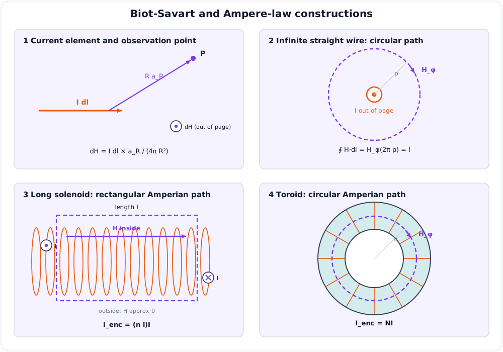
Application 1 - Infinite Straight Wire
Choose a circular Amperian path of radius \(\rho\) around the wire.
By symmetry:
and \(H_\phi\) is constant on the circular path.
Using Ampere's law:
Application 2 - Long Solenoid
For a long solenoid with \(n\) turns per meter and current \(I\), choose a rectangular Amperian path with one side inside the solenoid and one side outside.
The outside field is approximately zero, and the inside field is nearly uniform.
Enclosed current:
Therefore:
Application 3 - Toroid
For a toroid with \(N\) turns and current \(I\), choose a circular Amperian path of radius \(\rho\) inside the core.
Enclosed current is \(NI\).
Application 4 - Infinite Current Sheet
For an infinite sheet carrying surface current density \(\vec K = K\hat a_x\) on the plane \(z=0\), the magnetic field is uniform on both sides and opposite in direction.
Using Ampere's law:
The direction is obtained from the right-hand rule.
6. Curl and Point Form of Ampere's Law
Likely Exam Question (10 marks)
"Derive the point form of Ampere's circuital law and explain the physical meaning of curl."
Stokes' Theorem
Stokes' theorem relates the line integral of a vector field around a closed path to the surface integral of the curl of that field over any surface bounded by the path.
Apply Stokes' theorem to Ampere's circuital law:
Using Stokes' theorem:
Since this is true for any surface:
This is Ampere's law in differential form for magnetostatics.
Curl: Meaning
Curl measures the local rotation or circulation of a vector field.
- If \(\nabla \times \vec H \ne 0\), the magnetic field has local circulation.
- In magnetostatics, local circulation of \(\vec H\) is caused by current density \(\vec J\).
- Where there is no current density, \(\nabla \times \vec H = 0\), even though \(\vec H\) may still exist due to currents elsewhere.
Curl in Cartesian Coordinates
For:
Relation Between Curl and Current Density
If \(\vec H\) is known, current density can be found from:
Example:
If \(\vec H = 5x\hat a_y\,\text{A/m}\):
So:
7. Magnetic Flux and Gauss' Law for Magnetism
Magnetic Flux
Magnetic flux through a surface is:
Unit: weber (Wb)
Gauss' Law for Magnetism
Magnetic flux through any closed surface is zero:
Differential form:
Physical meaning:
- There are no isolated magnetic charges or monopoles in classical electromagnetics.
- Magnetic field lines always form closed loops.
- As much magnetic flux enters a closed surface as leaves it.
8. Magnetic Vector Potential
Likely Exam Question (5 marks)
"Define magnetic vector potential and state its relation with magnetic flux density."
Since:
magnetic flux density can be expressed as the curl of another vector field:
where \(\vec A\) is called the magnetic vector potential.
For a line current:
For volume current density:
Vector potential is especially useful for solving radiation, waveguide, and antenna problems.
9. Magnetic Energy and Inductance
Magnetic Energy Density
Energy stored per unit volume in a magnetic field is:
For a linear medium:
Total magnetic energy:
Inductance
Inductance is the flux linkage per unit current.
Unit: henry (H)
Energy stored in an inductor:
For a long solenoid:
where:
- \(N\) = number of turns
- \(A\) = cross-sectional area
- \(l\) = length of solenoid
10. Magnetic Boundary Conditions
At the boundary between two magnetic media, magnetic fields satisfy boundary conditions.
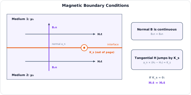
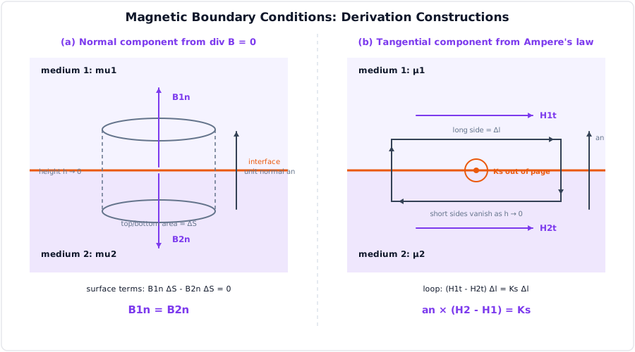
Normal Component of \(\vec B\)
From \(\nabla \cdot \vec B = 0\):
The normal component of magnetic flux density is continuous across the boundary.
Tangential Component of \(\vec H\)
From Ampere's law:
where \(\vec K_s\) is surface current density at the boundary.
If there is no surface current:
11. Solved Examples
Example 1 - Field Around a Long Straight Wire
Q. A long straight conductor carries \(10\,\text{A}\). Find \(H\) and \(B\) at a distance of \(5\,\text{cm}\) in free space.
Solution:
Example 2 - Magnetic Field at Center of Circular Coil
Q. A circular coil has 50 turns, radius \(10\,\text{cm}\), and current \(2\,\text{A}\). Find \(H\) at the center.
Solution:
Example 3 - Toroid Field
Q. A toroid has 400 turns and carries \(3\,\text{A}\). Find \(H\) at mean radius \(8\,\text{cm}\).
Solution:
Example 4 - Current Density from Curl of \(\vec H\)
Q. In a region, \(\vec H = (3y\hat a_x + 2x\hat a_y)\,\text{A/m}\). Find \(\vec J\).
Solution:
Only the \(z\)-component exists:
12. Quick Revision Table
| Topic | Key Result |
|---|---|
| Lorentz force | \(\vec F = Q(\vec E + \vec u \times \vec B)\) |
| Force on conductor | \(d\vec F = I\,d\vec l \times \vec B\) |
| Magnetic flux density | \(\vec B = \mu\vec H\) |
| Biot-Savart law | \(d\vec H = \frac{I\,d\vec l \times \hat a_R}{4\pi R^2}\) |
| Infinite wire | \(H = I/(2\pi\rho)\) |
| Circular loop center | \(H = NI/(2a)\) |
| Ampere's law | \(\oint_C \vec H \cdot d\vec l = I_{\text{enc}}\) |
| Point form of Ampere's law | \(\nabla \times \vec H = \vec J\) |
| Gauss law for magnetism | \(\nabla \cdot \vec B = 0\) |
| Vector potential | \(\vec B = \nabla \times \vec A\) |
| Magnetic energy density | \(w_m = \frac{1}{2}\mu H^2\) |
| Inductance | \(L = N\Phi/I\) |
Key Exam Points - Magnetostatics
- Use Biot-Savart's law for direct field calculation from current elements.
- Use Ampere's circuital law when symmetry makes \(\vec H\) constant along an Amperian path.
- The point form of Ampere's law is \(\nabla \times \vec H = \vec J\).
- Curl represents circulation per unit area; current density is the source of magnetic-field circulation.
- Magnetic flux lines are closed loops, so \(\nabla \cdot \vec B = 0\).
Model Answer — Biot-Savart and Ampere Laws with Applications [5 marks]
Exam-ready answer
Assume steady currents in a linear medium. For an oriented source element \(I\,d\vec l'\) at \(\vec r'\), define \(\vec R=\vec r-\vec r'\), \(R=|\vec R|\), and \(\hat a_R\) from the source element to the field point. The Biot-Savart law is
where \([H]=\text{A/m}\) and \(\vec B=\mu\vec H\) in tesla. The cross product and right-hand rule set the field direction. For a distributed current, replace \(I\,d\vec l'\) by \(\vec J\,dv'\) or \(\vec K\,dS'\) as appropriate.
Ampere's circuital law states
The positive normal to \(S\) is related to the positive traversal of \(C\) by the right-hand rule; a current through \(S\) along that normal is positive. Biot-Savart directly sums source contributions and works for arbitrary steady-current geometry, whereas Ampere's law becomes a practical field-solving method only when symmetry makes \(H\) constant or zero on sections of the path.
Biot-Savart application: at the centre of a circular loop of radius \(a\), every element has \(R=a\) and \(d\vec l'\perp\hat a_R\). All contributions point along the loop axis, so
Ampere-law application: for a long solenoid of \(N\) turns and length \(\ell\), a rectangular path enclosing \(NI\) gives \(H\ell=NI\) because the outside field and transverse contributions are negligible:
For example, \(N=500\), \(\ell=0.25\,\text{m}\) and \(I=0.10\,\text{A}\) give \(H=200\,\text{A/m}\). Finite solenoids have end fringing, and neither ideal result includes nonlinear saturation when \(\mu\) depends on \(H\). Applications include coils, electromagnets, current sensors and inductors.
Practice target: 9 minutes; state both orientation rules and derive one compact application of each law.
Model Answer — Ampere-Law Fields of a Wire, Solenoid, and Toroid [5 marks]
Exam-ready answer
For steady current, choose the contour direction first; the right-hand rule then defines the positive surface normal and enclosed current in
Infinite straight conductor: let current \(I\) flow in \(+\hat a_z\). Cylindrical symmetry gives \(\vec H=H_\phi\hat a_\phi\), counter-clockwise when viewed from \(+z\). On a circular path of radius \(\rho\),
Long solenoid: for \(N\) turns over length \(\ell\), use a rectangular contour with one side inside along the axis. The outside field is approximately zero and the short sides are normal to \(\vec H\), hence
with direction set by curled fingers following winding current; \(H_{\rm outside}\simeq0\) away from the ends.
Toroid: for \(N\) turns carrying \(I\), choose a circular path of radius \(\rho\) within a core of inner radius \(a\) and outer radius \(b\). Symmetry gives azimuthal \(\vec H\):
For an ideal tightly wound toroid, \(H\simeq0\) in the central hole \(\rho<a\) and outside \(\rho>b\), because an appropriate spanning surface encloses zero net linked current. In each linear material, \(\vec B=\mu\vec H\) T.
Check: for \(I=2\,\text{A}\) at \(\rho=0.10\,\text{m}\), the wire field is \(H=2/(2\pi\times0.10)=3.18\,\text{A/m}\). Doubling distance halves it. The wire result has \(1/\rho\) variation, the ideal solenoid is nearly uniform, and the toroid varies as \(1/\rho\) but confines flux. Finite length, sparse winding, leakage, fringing and core saturation limit the ideal formulas.
Practice target: 9 minutes; draw each Amperian path, mark the positive current, and show which path sections contribute.
Model Answer — Curl and the Point Form of Ampere's Law [5 marks]
Exam-ready answer
The curl of a vector field is the limiting circulation per unit area. If an infinitesimal surface has normal \(\hat n\) and its boundary is traversed by the right-hand rule,
Thus curl points along the axis about which circulation is greatest, with units A/m\(^2\) for \(\nabla\times\vec H\). In Cartesian coordinates,
Start with Ampere's circuital law for a steady current:
Stokes' theorem changes the left side to \(\int_S(\nabla\times\vec H)\cdot d\vec S\). Therefore
Since this holds for every oriented surface,
Physically, conduction current density is the local source of magnetic-field circulation; this differs from electrostatic \(\nabla\times\vec E=0\). It is also different from divergence: \(\nabla\cdot\vec B=0\) expresses no magnetic monopoles, while curl describes rotation.
Worked check: a solid cylindrical conductor carrying uniform \(\vec J=J_0\hat a_z\) has, by Ampere's law, \(H_\phi(2\pi\rho)=J_0\pi\rho^2\), so \(H_\phi=J_0\rho/2\) inside. In cylindrical coordinates,
which verifies the point law and direction. For time-varying fields the limitation is important: displacement current must be included, giving \(\nabla\times\vec H=\vec J+\partial\vec D/\partial t\). Curl is used in current-density recovery, field solvers and Maxwell-equation boundary analysis.
Practice target: 8–9 minutes; tie the contour orientation to the surface normal and verify the result inside a uniform-current conductor.
Model Answer — Scalar and Vector Magnetic Potentials [5 marks]
Exam-ready answer
A magnetic potential replaces a vector field by derivatives of a simpler unknown, but the scalar and vector forms follow from different field equations.
Scalar magnetic potential \(V_m\). In a current-free, simply connected magnetostatic region, \(\vec J=0\), so \(\nabla\times\vec H=0\). A curl-free field can be written
The minus sign makes \(\vec H\) point toward decreasing scalar potential. If \(\mu\) is constant, \(\nabla\cdot\vec B=\nabla\cdot(\mu\vec H)=0\) gives \(\nabla^2V_m=0\). The description is not globally single-valued around a current-carrying conductor: a loop linking current has \(\oint\vec H\cdot d\vec l=I\ne0\), contradicting the integral of a single-valued gradient.
Magnetic vector potential \(\vec A\). Since magnetic flux has zero divergence everywhere, \(\nabla\cdot\vec B=0\), it can always be represented locally as a curl:
For a homogeneous linear medium, substitute this relation into \(\nabla\times\vec H=\vec J\) and use \(\vec H=\vec B/\mu\):
With the Coulomb gauge \(\nabla\cdot\vec A=0\) and \(\nabla\times\nabla\times\vec A=\nabla(\nabla\cdot\vec A)-\nabla^2\vec A\),
For filamentary current, \(\vec A=(\mu I/4\pi)\int d\vec l'/R\), with \(d\vec l'\) following current direction. Taking its curl gives the physical \(\vec B\).
| Feature | Scalar \(V_m\) | Vector \(\vec A\) |
|---|---|---|
| Field obtained | \(\vec H=-\nabla V_m\) | \(\vec B=\nabla\times\vec A\) |
| Validity | Current-free simply connected region | Regions containing or excluding current |
| Governing form | Usually Laplace equation | Vector Poisson equation under a gauge |
| Non-uniqueness | Additive constant | Gauge: \(\vec A+\nabla\chi\) gives the same \(\vec B\) |
Check/application: for a uniform \(\vec B=B_0\hat a_z\), choosing \(\vec A=\tfrac12B_0\rho\hat a_\phi\) gives \((\nabla\times\vec A)_z=(1/\rho)d(\rho A_\phi)/d\rho=B_0\). Scalar potential is efficient in air gaps and magnetic circuits; vector potential is preferred for coils, inductance, flux linkage and finite-element analysis.
Practice target: 9 minutes; organize the answer as curl-free H versus divergence-free B, then state domain and uniqueness limitations.
Model Answer — Magnetic Boundary Conditions [5 marks]
Exam-ready answer
Let an interface separate media 1 and 2, and define the unit normal \(\hat n\) to point from medium 1 into medium 2. Let a free surface-current sheet \(\vec K_s\) in A/m lie tangentially on the interface.
Normal component of \(\vec B\). Apply Gauss's law for magnetism to a thin pillbox of face area \(\Delta S\) and height tending to zero:
Side flux vanishes with height. The upper face contributes \(B_{2n}\Delta S\) and the lower outward face contributes \(-B_{1n}\Delta S\), so
or \(B_{2n}=B_{1n}\). There is no magnetic surface charge. For linear media this becomes
Tangential component of \(\vec H\). Apply Ampere's law to an infinitesimal rectangular loop straddling the boundary. The two short normal sides vanish. Choosing its traversal consistently with the right-hand rule, the enclosed sheet current is \(\vec K_s\) projected across the loop, giving the vector result
Equivalently, for a tangent \(\hat t\) normal to \(\vec K_s\) in the surface, the signed jump is fixed by the chosen \(\hat n,\hat t\) orientation. If \(\vec K_s=0\),
Check: at a current-free boundary with \(\mu_2=4\mu_1\), continuity of normal \(B\) requires \(H_{2n}=H_{1n}/4\), while tangential \(H\) remains unchanged. Hence field lines refract according to \(\tan\theta_2/\tan\theta_1=\mu_2/\mu_1\) when \(\theta\) is measured from the normal. These conditions are used at air gaps, magnetic cores, shielding surfaces and waveguide walls. They assume an ideal zero-thickness interface; finite transition layers and nonlinear or hysteretic media require their local constitutive \(B(H)\) relation, but the integral boundary laws remain valid.
Practice target: 9 minutes; draw both infinitesimal constructions, mark the 1-to-2 normal, and retain the cross-product order.