Series and Parallel Resonant Circuits¶

Possible Exam Questions¶

Exam Questions and Answer Map

Explain series and parallel resonance. Derive resonant frequency, quality factor and bandwidth, and compare the two circuits. [10] — [likely]
Answer plan: Define reactive cancellation → write series impedance and parallel admittance → identify extrema/current/voltage magnification → derive resistance-specific \(Q\) → obtain \(BW=f_0/Q\) → compare and apply.
Model answer: Series and Parallel Resonance, Q and Bandwidth

1. Resonance Concept¶

Resonance is the frequency at which inductive and capacitive reactive effects cancel at the circuit terminals. For ideal \(L,C\),

\[ X_L=X_C, \]

\[ \omega_0L=\frac{1}{\omega_0C}, \]

\[ \boxed{f_0=\frac{1}{2\pi\sqrt{LC}}}. \]

At resonance the terminal impedance/admittance is purely real, but series and parallel connections produce opposite terminal behaviour.

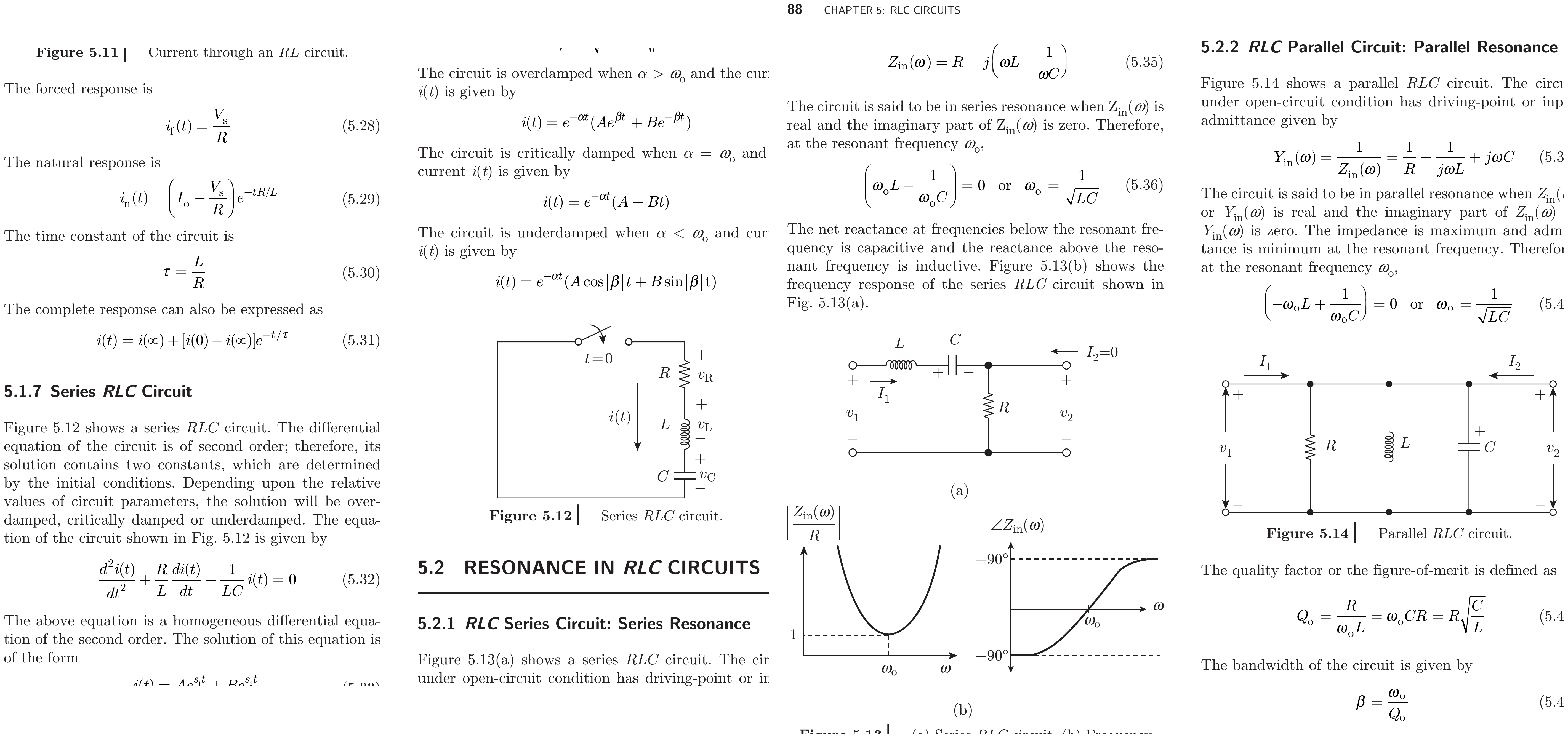
Fig: Textbook series- and parallel-resonance circuits and responses

2. Series Resonance¶

For total series resistance \(R_s\),

\[ Z_s=R_s+j\left(\omega L-\frac{1}{\omega C}\right). \]

At Parallel Resonance¶

\[ Z_s(\omega_0)=R_s. \]

terminal impedance is minimum;
source current \(I=V/R_s\) is maximum;
source power factor is unity;
\(V_L\) and \(V_C\) are equal in magnitude, opposite in phase and can greatly exceed source voltage.

The series quality factor is

\[ \boxed{Q_s=\frac{\omega_0L}{R_s} =\frac{1}{\omega_0CR_s} =\frac{1}{R_s}\sqrt{\frac{L}{C}}}. \]

At resonance,

\[ V_L=IX_L=Q_sV, \qquad V_C=IX_C=Q_sV. \]

This is voltage magnification. The large internal voltages cancel at the source terminals but still stress components.

3. Series Half-Power Bandwidth¶

At half power, current falls to \(I_{max}/\sqrt2\), so

\[ \left\lvert\omega L-\frac{1}{\omega C}\right\rvert=R_s. \]

The exact series-RLC angular bandwidth is

\[ \Delta\omega=\omega_2-\omega_1=\frac{R_s}{L}. \]

Since \(Q_s=\omega_0L/R_s\),

\[ \boxed{BW=f_2-f_1=\frac{f_0}{Q_s}}. \]

Also, for ideal series RLC,

\[ f_1f_2=f_0^2. \]

Fig: Textbook resonance response and bandwidth relations

4. Ideal Parallel Resonance¶

For ideal \(L,C\) and a parallel resistance \(R_p\),

\[ Y_p=\frac{1}{R_p}+j\left(\omega C-\frac{1}{\omega L}\right). \]

At Resonance¶

\[ Y_p(\omega_0)=\frac{1}{R_p}, \qquad Z_p(\omega_0)=R_p. \]

terminal admittance is minimum and impedance maximum;
source/line current is minimum;
inductor and capacitor branch currents are large, equal and opposite at the terminals;
energy circulates inside the tank.

The parallel quality factor is

\[ \boxed{Q_p=\frac{R_p}{\omega_0L} =\omega_0CR_p =R_p\sqrt{\frac{C}{L}}}. \]

At resonance, reactive branch current relative to line-loss current is

\[ \frac{I_C}{I_R}=\omega_0CR_p=Q_p, \]

which is current magnification.

5. Practical Parallel Tank with Coil Loss¶

A physical inductor often has series resistance \(r_s\). For the branch \(r_s+j\omega L\) in parallel with \(C\), resonance occurs when total susceptance is zero. For high \(Q\),

\[ f_r\approx\frac{1}{2\pi\sqrt{LC}}, \]

\[ \boxed{Q\approx\frac{\omega_0L}{r_s}}, \]

and the dynamic parallel resistance near resonance is

\[ \boxed{R_{p,eq}\approx\frac{(\omega_0L)^2}{r_s} =\frac{L}{Cr_s}}. \]

Do not insert the coil's small series \(r_s\) into the ideal parallel formula \(Q_p=R_p\sqrt{C/L}\); they are different equivalent models.

6. Bandwidth and Selectivity¶

For either standard high-\(Q\) resonator under its corresponding driven response,

\[ \boxed{Q=\frac{f_0}{BW}}, \qquad \boxed{BW=f_2-f_1}. \]

Higher \(Q\) means lower fractional energy loss per cycle.
Higher \(Q\) gives narrower bandwidth and sharper selectivity.
Higher \(Q\) also increases internal voltage/current stress and settling time.

Selectivity is the ability to accept the desired frequency and reject nearby frequencies.

7. Series vs Parallel Comparison¶

Property	Series resonance	Parallel resonance
Terminal impedance at \(f_0\)	Minimum, \(R_s\)	Maximum, \(R_p\) in ideal parallel model
Supply current	Maximum	Minimum
Internal magnification	Voltage across \(L,C\)	Circulating branch current
Ideal resistance model	Series \(R_s\)	Parallel \(R_p\)
Common use	Frequency-selective current path, matching	Oscillator/tuned-amplifier tank, high-impedance load

A series resonator often forms a pass path and a parallel resonator often a reject/high-impedance path, but band-pass versus band-stop depends on circuit placement and where output is measured, not on the resonator name alone.

8. Applications¶

Series Resonance¶

Band-selection paths, impedance matching, series-tuned antennas, induction heating and frequency measurement.

Parallel Resonance¶

Oscillator tanks, collector/drain loads in tuned amplifiers, RF traps, receiver selection and impedance transformation.

Exam Traps

Series resonance: minimum \(Z\), maximum source current.
Parallel resonance: maximum \(Z\), minimum source current.
Name the resistance model before writing \(Q\).
Half-power means power \(1/2\), current/voltage response magnitude \(1/\sqrt2\) in the relevant driven response.

Rapid Recall¶

\(f_0=1/(2\pi\sqrt{LC})\).
Series: \(Q_s=\omega_0L/R_s\).
Ideal parallel: \(Q_p=R_p/(\omega_0L)\).
Coil loss: \(Q\approx\omega_0L/r_s\).
\(Q=f_0/BW\).

Model Answer — Series and Parallel Resonance, Q and Bandwidth [10 marks]¶

Exam-ready answer

Resonance occurs when inductive and capacitive reactive effects cancel:

\[ \omega_0L=\frac1{\omega_0C} \quad\Rightarrow\quad \boxed{f_0=\frac1{2\pi\sqrt{LC}}}. \]

For series resistance \(R_s\),

\[ Z_s=R_s+j\left(\omega L-\frac1{\omega C}\right). \]

At \(f_0\), impedance is minimum \(R_s\), current maximum and power factor unity. Equal opposite \(V_L,V_C\) may each equal \(Q_sV\) (voltage magnification), where

\[ \boxed{Q_s=\frac{\omega_0L}{R_s} =\frac1{\omega_0CR_s}}. \]

For ideal parallel \(R_p,L,C\),

\[ Y_p=\frac1{R_p}+j\left(\omega C-\frac1{\omega L}\right). \]

At \(f_0\), admittance is minimum, impedance maximum \(R_p\) and line current minimum; equal opposite \(L,C\) branch currents circulate. Its quality factor is

\[ \boxed{Q_p=\frac{R_p}{\omega_0L}=\omega_0CR_p}. \]

If coil loss is instead series \(r_s\), use \(Q\approx\omega_0L/r_s\) and \(R_{p,eq}\approx L/(Cr_s)\) for high \(Q\); do not mix models.

At half-power frequencies \(f_1,f_2\), response magnitude is \(1/\sqrt2\) of its resonant value, and

\[ \boxed{BW=f_2-f_1=\frac{f_0}{Q}}. \]

Higher \(Q\) means lower loss, narrower bandwidth and better selectivity, but higher internal stress and slower settling. Series resonance is used in selective current paths/matching; parallel resonance in oscillator and tuned-amplifier tanks. Filter action still depends on placement and output measurement.

Practice target: 18 minutes; derive series impedance and parallel admittance, write resistance-specific \(Q\) formulas, compare extrema/magnification and calculate one \(f_0,Q,BW\) example.