Root Locus Method
Possible Exam Questions
Exam Questions and Answer Map
Questions labelled [PYQ paper/year] are observed past questions; those labelled [likely] are pattern-based predictions. For each one, rehearse the answer plan closed-book, then use the links to verify the full answer in this chapter.
-
What is the root locus? State the rules for constructing a root locus. [5–10] — [likely]
-
Answer plan: Define root locus → state angle and magnitude conditions → enumerate 10 construction rules (branches, start/end, symmetry, real-axis segments, asymptotes, breakaway, departure angle, arrival angle, jω crossing, gain formula).
-
Model answer: Root-locus definition and construction rules
-
For a given G(s)H(s), sketch the root locus for 0 ≤ K ≤ ∞ and find the breakaway point and the angle of departure. [6+4=10] — [PYQ 2081]
-
Answer plan: Identify open-loop poles/zeros → determine real-axis segments → calculate asymptote angles and centroid → solve \(dK/ds=0\) for breakaway point → compute angle of departure from complex pole using \(\phi_d = 180° + \Sigma\angle(\text{zeros}) - \Sigma\angle(\text{other poles})\) → sketch complete locus.
-
Model answer: NTC 2081 parameterized root-locus construction
-
How is the root locus used to determine stability and the value of K for marginal stability? [5] — [likely]
-
Answer plan: Explain that stability requires all closed-loop poles in LHP → find jω-axis crossing using Routh-Hurwitz or substituting \(s=j\omega\) → value of \(K\) at crossing is marginal-stability gain → for \(K\) below this value system is stable.
- Model answer: Root locus, stability range, and marginal gain
Syllabus Focus
- Root locus method
- Closed-loop pole movement with gain variation
- Stability from root locus
- Root locus construction rules
- Transient-response interpretation from pole locations
1. Introduction to Root Locus
Likely Exam Question (5 marks)
"Define root locus. Why is it useful in control-system analysis and design?"
The root locus is the path traced by the roots of the closed-loop characteristic equation as a system parameter, usually gain \(K\), varies from \(0\) to \(\infty\).
For a negative-feedback system:
The characteristic equation is:
The root locus shows how the closed-loop poles move in the \(s\)-plane as \(K\) changes.
Importance
Root locus helps determine:
- Stability range of gain \(K\)
- Transient response as gain changes
- Dominant closed-loop pole locations
- Damping ratio and natural frequency
- Effect of adding poles and zeros
- Controller or compensator design
Basic Idea
Open-loop poles and zeros determine the possible paths of closed-loop poles.
As \(K\) changes:
- Closed-loop poles start at open-loop poles when \(K=0\).
- Closed-loop poles end at open-loop zeros or infinity when \(K\to\infty\).
2. Characteristic Equation and Root Locus Conditions
Likely Exam Question (10 marks)
"Derive the angle and magnitude conditions for root locus."
For negative feedback:
Therefore:
Since \(-1\) has magnitude 1 and angle odd multiples of \(180^\circ\):
These are the two root locus conditions.
Angle Condition
A point \(s=s_0\) lies on the root locus if:
where:
- \(z_i\) = open-loop zeros
- \(p_i\) = open-loop poles
Magnitude Condition
Once a point is known to lie on root locus, the gain \(K\) at that point is:
assuming open-loop transfer function is:
3. Root Locus Construction Rules
Likely Exam Question (10 marks)
"State the rules for constructing root locus and sketch the root locus for a given transfer function."
Consider:
Let:
- \(n\) = number of open-loop poles
- \(m\) = number of open-loop zeros
Rule 1 - Number of Branches
The number of root locus branches equals the number of open-loop poles.
Rule 2 - Starting and Ending Points
- Root locus starts at open-loop poles when \(K=0\).
- Root locus ends at open-loop zeros when \(K\to\infty\).
- If \(n>m\), then \(n-m\) branches end at infinity.
Rule 3 - Symmetry
Root locus is symmetric about the real axis because complex roots occur in conjugate pairs.
Rule 4 - Real-Axis Segments
A point on the real axis lies on the root locus if the total number of open-loop poles and zeros to its right is odd.
Rule 5 - Asymptotes
If \(n>m\), then \(n-m\) branches go to infinity along asymptotes.
Number of asymptotes:
Angles of asymptotes:
Centroid of asymptotes:
where sums are algebraic sums of pole and zero locations.
Rule 6 - Breakaway and Break-In Points
Breakaway points occur where branches leave the real axis.
Break-in points occur where branches enter the real axis.
From characteristic equation:
Solve for \(K\) as a function of \(s\):
Break points are found from:
Only points that lie on valid real-axis root locus segments are accepted.
Rule 7 - Angle of Departure from Complex Poles
For a complex pole \(p_k\), angle of departure is:
Rule 8 - Angle of Arrival at Complex Zeros
For a complex zero \(z_k\), angle of arrival is:
Rule 9 - Imaginary-Axis Crossing
The points where root locus crosses the imaginary axis are found using the Routh-Hurwitz criterion on the characteristic equation.
At crossing, substitute \(s=j\omega\) or use the auxiliary equation from the Routh array.
Rule 10 - Gain at Any Point
Use magnitude condition:
4. Root Locus and Stability
Likely Exam Question (10 marks)
"Use root locus to determine the range of gain for system stability."
A continuous-time closed-loop system is stable if all closed-loop poles lie in the left half of the \(s\)-plane.
Root locus shows the closed-loop pole locations for all values of gain \(K\).
Stability from Root Locus
| Root Locus Location | Stability |
|---|---|
| All branches in LHP | Stable for corresponding \(K\) |
| Any branch crosses into RHP | Unstable beyond crossing gain |
| Branch on imaginary axis | Marginally stable at that gain |
Gain Range
To find stable gain range:
- Write characteristic equation \(1+KG(s)H(s)=0\).
- Apply Routh-Hurwitz criterion.
- Find range of \(K\) for which all first-column elements are positive.
- Imaginary-axis crossing gain matches root locus crossing.
5. Routh-Hurwitz Criterion for Root Locus Support
Likely Exam Question (10 marks)
"Determine stability range using Routh-Hurwitz criterion."
For characteristic equation:
construct the Routh array. The system is stable if all elements in the first column have the same sign and none are zero.
Routh Array Structure
For a fourth-order equation:
Routh table:
| Power | First Column | Second Column | Third Column |
|---|---|---|---|
| \(s^4\) | \(a_4\) | \(a_2\) | \(a_0\) |
| \(s^3\) | \(a_3\) | \(a_1\) | \(0\) |
| \(s^2\) | \(b_1\) | \(b_2\) | \(0\) |
| \(s^1\) | \(c_1\) | \(0\) | \(0\) |
| \(s^0\) | \(a_0\) | \(0\) | \(0\) |
where:
Interpretation
Number of sign changes in the first column equals the number of roots in the right half-plane.
Special cases:
- Zero in first column: replace by small \(\epsilon\) and continue.
- Entire row zero: use auxiliary equation from the row above and differentiate it.
6. Root Locus and Transient Response
Likely Exam Question (5 marks)
"Explain how root locus is used to study transient response."
Closed-loop pole locations determine transient response.
For dominant complex poles:
Natural frequency:
Damping ratio:
Settling time:
Peak time:
Percent overshoot:
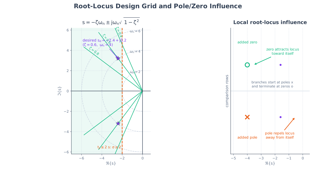
Constant Damping Ratio Lines
Lines of constant damping ratio are radial lines from the origin.
If the angle from the negative real axis is \(\theta\):
Constant Natural Frequency Circles
Lines of constant natural frequency are circles centered at the origin:
Constant Settling Time Lines
Settling time depends on real part \(\sigma\):
Thus constant settling time lines are vertical lines in the left half-plane.
7. Effect of Adding Poles and Zeros
Likely Exam Question (5 marks)
"Explain the effect of adding open-loop poles and zeros on root locus and system response."
Adding an Open-Loop Pole
Adding a pole tends to pull the root locus toward the right half-plane.
Effects:
- Decreases relative stability
- Slows response
- Increases overshoot
- Can make system unstable
Adding an Open-Loop Zero
Adding a zero tends to pull the root locus toward the left half-plane.
Effects:
- Improves relative stability
- Speeds up response
- Can reduce settling time
- Often used in lead compensation
Compensator Interpretation
| Compensator | Root Locus Effect | Main Purpose |
|---|---|---|
| Lead compensator | Adds zero closer to origin than pole | Improves transient response and stability margin |
| Lag compensator | Adds pole closer to origin than zero | Improves steady-state accuracy |
| PID controller | Adds pole/zeros depending on settings | Improves both transient and steady-state response |
8. Root Locus Design Procedure
Likely Exam Question (10 marks)
"Design the gain of a control system using root locus to satisfy damping ratio or settling time requirements."
Typical design steps:
- Write open-loop transfer function \(G(s)H(s)\).
- Plot open-loop poles and zeros.
- Sketch root locus using construction rules.
- Translate time-domain specifications into desired pole region.
- Choose desired dominant pole location on the root locus.
- Use magnitude condition to calculate gain \(K\).
- Verify remaining poles are non-dominant.
- If root locus does not pass through desired point, add compensator.
Desired Pole from Specifications
If percent overshoot is specified, find \(\zeta\):
If settling time is specified:
Desired dominant poles are:
or:
9. Solved Examples
NTC 2081 PYQ - Parameterized Four-Pole Root Locus
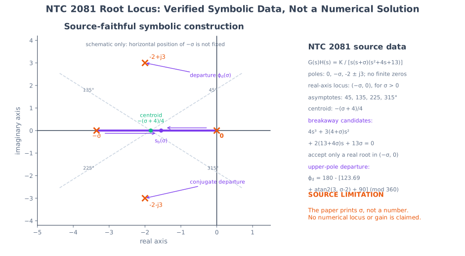
The source paper gives:
Its open-loop poles are:
There are four branches and no finite zeros. Therefore the four asymptote angles are:
and the centroid is:
The real-axis locus lies between the two real poles \(-\sigma\) and \(0\). From
the breakaway candidates satisfy:
Only a real root lying in \((-\sigma,0)\) is a valid breakaway point. For the upper complex pole, the angle of departure is:
The lower-pole departure angle is its complex-conjugate reflection.
Source-paper limitation
The repository scan itself prints the parameter \(\sigma\), not a numeral, and supplies no later value for it. Therefore the exact breakaway coordinate and departure angle must remain functions of \(\sigma\); this is a verified symbolic transcription, not a verified numerical solution.
Example 1 - Basic Root Locus Data
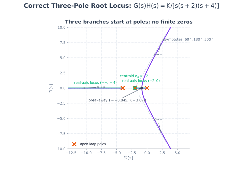
Q. For \(G(s)H(s)=\frac{K}{s(s+2)(s+4)}\), find number of branches, real-axis segments, asymptote angles, and centroid.
Solution:
Open-loop poles: \(0,-2,-4\)
Open-loop zeros: none
Number of branches:
Real-axis segments exist where the number of poles/zeros to the right is odd:
- \((-\infty,-4)\): 3 to the right → root locus exists
- \((-4,-2)\): 2 to the right → no root locus
- \((-2,0)\): 1 to the right → root locus exists
- \((0,\infty)\): 0 to the right → no root locus
Asymptotes:
Centroid:
Example 2 - Breakaway Point
Q. For \(G(s)H(s)=\frac{K}{s(s+4)}\), find the breakaway point.
Solution:
Characteristic equation:
Breakaway point:
This point lies between poles at \(0\) and \(-4\), which is a valid root-locus segment.
Example 3 - Stability Range Using Routh
Q. Find range of \(K\) for stability if characteristic equation is:
Solution:
Routh array:
| Power | First Column | Second Column |
|---|---|---|
| \(s^3\) | 1 | 11 |
| \(s^2\) | 6 | \(6+K\) |
| \(s^1\) | \(\frac{6(11)-(6+K)}{6}\) | 0 |
| \(s^0\) | \(6+K\) | 0 |
For stability, first column must be positive:
For positive gain:
Example 4 - Gain at Desired Pole
Q. For \(G(s)H(s)=\frac{K}{s(s+2)}\), find gain \(K\) when closed-loop pole is at \(s=-1+j2\).
Solution:
Use magnitude condition:
At \(s=-1+j2\):
10. Quick Revision Table
| Topic | Key Result |
|---|---|
| Characteristic equation | \(1+KG(s)H(s)=0\) |
| Angle condition | \(\angle G(s)H(s)=(2q+1)180^\circ\) |
| Magnitude condition | \(\lvert KG(s)H(s)\rvert=1\) |
| Number of branches | Number of open-loop poles |
| Branch start | Open-loop poles |
| Branch end | Open-loop zeros or infinity |
| Real-axis rule | Odd number of poles/zeros to the right |
| Number of asymptotes | \(n-m\) |
| Asymptote angles | \(\theta_q=(2q+1)180^\circ/(n-m)\) |
| Centroid | \(\sigma_a=(\sum p_i-\sum z_i)/(n-m)\) |
| Breakaway points | \(dK/ds=0\) |
| Stability crossing | Use Routh-Hurwitz criterion |
| Constant damping line | \(\zeta=\cos\theta\) |
| Constant settling-time line | Vertical line \(\sigma=4/t_s\) |
Key Exam Points - Root Locus
- Root locus shows closed-loop pole movement as gain \(K\) varies from \(0\) to \(\infty\).
- It starts at open-loop poles and ends at open-loop zeros or infinity.
- A real-axis point is on root locus if the number of open-loop poles/zeros to its right is odd.
- Use Routh criterion to find imaginary-axis crossing and stable gain range.
- Adding a zero usually improves relative stability; adding a pole usually reduces it.
Model Answer — Root-Locus Definition and Construction Rules [10 marks]
Exam-ready answer
For a negative-feedback LTI system, write the characteristic equation as
where \(L_0(s)=G(s)H(s)\) excludes the variable real gain \(K\). The root locus is the set of all closed-loop pole positions in the \(s\)-plane as \(K\) varies from \(0\) to \(\infty\). The horizontal axis is \(\sigma\) in s\(^{-1}\) and the vertical axis is \(j\omega\) in rad/s.
Rearranging gives \(KL_0(s)=-1=1\angle(2q+1)180^\circ\). Therefore a point belongs to the positive-\(K\) locus only if
and its gain is
If \(L_0=\prod_{i=1}^m(s-z_i)/\prod_{i=1}^n(s-p_i)\), use these construction rules:
- There are \(n\) branches, one for each open-loop pole.
- At \(K=0\) branches start at \(p_i\). As \(K\to\infty\), \(m\) end at finite zeros \(z_i\) and \(n-m\) end at infinity.
- With real coefficients, the locus is symmetric about the real axis.
- A real-axis point is on the positive-\(K\) locus if the number of real poles and zeros to its right is odd.
- The \(n-m\) asymptotes toward infinite zeros have
and intersect at
- On a real segment, write \(K(s)=-1/L_0(s)\) and solve \(dK/ds=0\) for breakaway or break-in candidates. Retain only points on a valid locus segment with \(K\ge0\).
- From a complex pole \(p_k\), the departure angle is
- At a complex zero \(z_k\), the arrival angle is found by applying the same angle condition while excluding that zero:
- Find imaginary-axis crossings and the associated \(K\) by Routh-Hurwitz or by substituting \(s=j\omega\) into the characteristic equation and equating real and imaginary parts.
- At any proposed point, use the magnitude condition, equivalently \(K=\prod|s-p_i|/\prod|s-z_i|\), and mark branch arrows from poles toward zeros as \(K\) increases.
Worked check: for \(KL_0=K/[s(s+2)(s+4)]\), poles are \(0,-2,-4\), there are no zeros, real segments are \((-2,0)\) and \((-\infty,-4)\), the centroid is \(-2\), and asymptote angles are \(60^\circ,180^\circ,300^\circ\). Since
the candidates are \(s=-2\pm2\sqrt3/3\). Only \(s=-0.845\) lies on a valid segment; \(s=-3.155\) lies in \((-4,-2)\) and must be rejected.
Root locus directly relates gain to stability, damping and speed, but it is based on the modeled pole-zero set, usually varies one scalar gain, and becomes cumbersome for delays or high-order uncertain plants. It guides compensator placement; final gain and robustness should be checked by Routh and frequency-response margins.
Practice target: 18–20 minutes; derive angle/magnitude conditions, list all ten rules, and validate one candidate rather than accepting every dK/ds root.
Model Answer — NTC 2081 Parameterized Root-Locus Construction [10 marks]
Exam-ready answer
The available NTC 2081 source states
and does not assign a numerical value to \(\sigma\). Assume only \(\sigma>0\) so \(-\sigma\) is a left-half-plane real pole. Negative feedback gives \(1+G(s)H(s)=0\) and \(K\ge0\).
Part A — Root-locus construction and breakaway [6 marks]
The open-loop poles are
with no finite zeros. Hence four branches start at these poles and all four end at infinity. The locus is conjugate-symmetric. On the real axis the only segment is between the two real poles, namely the open interval joining \(-\sigma\) and \(0\), because exactly one real pole lies to the right of each point there.
With \(n-m=4\), the asymptote angles and centroid are
From the characteristic equation,
The breakaway candidates satisfy \(dK/ds=0\):
Only a real root lying between \(-\sigma\) and \(0\) and producing \(K>0\) is a valid breakaway. Because its coordinate varies with the unspecified parameter, no unique decimal value can be reported.
Part B — Angle of departure [4 marks]
For the upper pole \(p_+=-2+j3\), measure all vectors from the other poles to \(p_+\). Their angles are
There are no zero angles. Applying the root-locus angle condition while excluding \(p_+\) gives
The lower-pole departure is the reflection across the real axis:
Consistency check: the conjugate pole sum is \(-4\), so the centroid numerator must be \(-(\sigma+4)\), and conjugate symmetry requires opposite departure angles. Once a numerical \(\sigma\) is supplied, solve the cubic, reject invalid candidates with the real-axis and \(K>0\) tests, evaluate the angle, and use \(K=|s(s+\sigma)(s^2+4s+13)|\) to label the sketch.
The symbolic result is the most specific answer justified by the source. Choosing a convenient \(\sigma\) would change the pole order, centroid, breakaway and departure angle and would therefore be technically dishonest. Root locus also represents the stated linear model only; unmodeled delay and parameter uncertainty still require robustness checks.
Practice target: 20 minutes; allocate about 12 minutes to the 6-mark construction/breakaway and 8 minutes to the 4-mark departure-angle geometry.
Model Answer — Root Locus, Stability Range, and Marginal Gain [5 marks]
Exam-ready answer
For negative feedback with characteristic equation
the points on the root locus are the closed-loop poles for each \(K\). A continuous-time rational system is asymptotically/BIBO stable when all branches for that gain lie strictly in the left half-plane. Their distance from the imaginary axis indicates relative stability: poles farther left generally decay faster, while a complex pole angle gives damping ratio \(\zeta=-\operatorname{Re}(p)/|p|\).
The gain at which a conjugate pair reaches \(s=\pm j\omega_c\) is the marginal-stability gain. Two standard procedures are:
- Form the polynomial \(D(s)+KN(s)=0\), substitute \(s=j\omega\), and solve simultaneous real and imaginary equations for \(K\) and \(\omega\).
- Construct the Routh array. Require every first-column term to have the same sign for stability. Set the row that reaches zero to its boundary value; the auxiliary polynomial from the row above gives \(\omega_c\).
Worked check: for
the characteristic polynomial is
Its Routh first column is
Therefore
At \(K=48\), the \(s^1\) row vanishes. The auxiliary equation from the \(s^2\) row is \(6s^2+48=0\), so
Indeed, the polynomial factors as \((s+6)(s^2+8)\), confirming one LHP pole and a simple imaginary pair. For \(K>48\), branches enter the RHP and the system is unstable. The statement “below marginal gain is stable” is not universal without checking all Routh inequalities; systems with RHP open-loop poles or multiple crossings can have several stable/unstable intervals. Root locus gives the geometry, while Routh gives an exact gain range for a polynomial model.
Practice target: 9 minutes; state the LHP condition, build the short Routh array, and verify the crossing with the auxiliary polynomial.