Electrostatics
Possible Exam Questions
Exam Questions and Answer Map
Questions labelled [PYQ paper/year] are observed past questions; those labelled [likely] are pattern-based predictions. For each one, rehearse the answer plan closed-book, then use the links to verify the full answer in this chapter.
-
State and explain Coulomb's law; define electric field intensity E. [5] — [likely]
-
Answer plan: State Coulomb's law in scalar and vector form → define \(\vec E\) as force per unit charge → derive \(\vec E\) from a point charge → mention superposition principle → state units.
-
Model answer: Coulomb's law and electric field intensity
-
Define electric flux and electric flux density D; relate D and E. [5] — [likely]
-
Answer plan: Define electric flux \(\Psi\) → define flux density \(\vec D\) → write \(\vec D = \epsilon\vec E\) → explain relation in free space and dielectric → introduce polarization vector.
-
Model answer: Electric flux, flux density, and the D-E relation
-
State Gauss's law; derive Maxwell's first equation (∇·D = ρ) using the divergence theorem. [5–10] — [likely]
-
Answer plan: State Gauss's law in integral form → apply divergence theorem to convert surface integral to volume integral → equate integrands → obtain \(\nabla\cdot\vec D = \rho_v\) → state physical meaning.
-
Model answer: Gauss's law and Maxwell's first equation
-
Use Gauss's law to find E for a point charge, an infinite line charge and a charged sphere. [5] — [likely]
-
Answer plan: Choose Gaussian surface for each geometry (sphere, cylinder, sphere) → apply symmetry → evaluate \(\oint \vec D\cdot d\vec S\) → solve for \(\vec E\) → state results.
-
Model answer: Fields from point, line, and spherical charges
-
Define electric potential; derive the relation E = −∇V. [5] — [likely]
-
Answer plan: Define potential as work per unit charge → write potential difference integral → differentiate to get \(\vec E = -\nabla V\) → give Cartesian expansion → mention equipotential surfaces.
-
Model answer: Electric potential and the field-gradient relation
-
Derive Laplace's and Poisson's equations and state their applications. [5] — [likely]
-
Answer plan: Start from \(\nabla\cdot\vec D = \rho_v\) and \(\vec E = -\nabla V\) → substitute to get Poisson's equation \(\nabla^2V = -\rho_v/\epsilon\) → set \(\rho_v = 0\) for Laplace → list common coordinate forms → state applications (capacitor, boundary-value problems).
- Model answer: Poisson's and Laplace's equations
Syllabus Focus
- Coulomb's law
- Electric field intensity
- Electric flux density
- Gauss' law
- Maxwell's first equation
- Divergence theorem
- Energy and potential
- Laplace and Poisson equations
1. Electric Charge and Coulomb's Law
Likely Exam Question (5 marks)
"State and explain Coulomb's law. Derive the expression for electric field intensity due to a point charge."
Electric Charge
Electric charge is the fundamental property responsible for electric force. It exists in two forms: positive and negative.
| Quantity | Symbol | Unit |
|---|---|---|
| Charge | \(Q\) | coulomb (C) |
| Elementary charge | \(e\) | \(1.602 \times 10^{-19}\,\text{C}\) |
| Permittivity of free space | \(\epsilon_0\) | \(8.854 \times 10^{-12}\,\text{F/m}\) |
Important properties:
- Quantization: \(Q = \pm ne\), where \(n\) is an integer.
- Conservation: total charge of an isolated system remains constant.
- Additivity: total charge is the algebraic sum of individual charges.
Coulomb's Law
Coulomb's law states that the force between two stationary point charges is directly proportional to the product of the charges and inversely proportional to the square of the distance between them.
For charges \(Q_1\) and \(Q_2\) separated by distance \(R\):
In vector form, the force on \(Q_2\) due to \(Q_1\) is:
where:
- \(\epsilon = \epsilon_0\epsilon_r\) is the permittivity of the medium.
- \(\hat a_{21}\) is the unit vector from \(Q_1\) to \(Q_2\).
- If \(Q_1Q_2 > 0\), the force is repulsive.
- If \(Q_1Q_2 < 0\), the force is attractive.
For free space:
Superposition Principle
If several point charges act on a charge \(Q\), the total force is the vector sum of forces due to each charge:
Electrostatic fields are linear, so the same superposition principle applies to electric field intensity and potential.
2. Electric Field Intensity
Likely Exam Question (5 marks)
"Define electric field intensity. Find the electric field due to point, line, surface, and volume charge distributions."
Definition
Electric field intensity is the force experienced by a unit positive test charge placed at a point in an electric field.
Unit:
Field Due to a Point Charge
For a point charge \(Q\) at the origin:
The field points radially outward for positive charge and radially inward for negative charge.
Field Due to Multiple Point Charges
For \(n\) charges:
Continuous Charge Distributions
Real charge may be distributed continuously over a line, surface, or volume.
| Distribution | Density | Unit | Charge Element |
|---|---|---|---|
| Line charge | \(\rho_l\) | C/m | \(dQ = \rho_l\,dl\) |
| Surface charge | \(\rho_s\) | C/m\(^2\) | \(dQ = \rho_s\,dS\) |
| Volume charge | \(\rho_v\) | C/m\(^3\) | \(dQ = \rho_v\,dv\) |
The electric field due to a continuous charge distribution is found by integration:
For each distribution:
Electric Field Lines
Electric field lines are imaginary lines used to represent the direction and relative strength of \(\vec E\).
- Lines start on positive charge and end on negative charge.
- Tangent at any point gives the direction of \(\vec E\).
- Closer spacing means stronger field.
- Field lines never cross.
3. Electric Flux and Electric Flux Density
Likely Exam Question (5 marks)
"Define electric flux density. Explain its relation with electric field intensity and charge."
Electric Flux
Electric flux represents the total electric field passing through a surface.
Unit: coulomb (C)
Electric Flux Density
Electric flux density is the electric flux per unit area normal to the direction of flux.
Unit:
For a point charge in a homogeneous medium:
Therefore:
Notice that \(\vec D\) due to a point charge is independent of the medium permittivity, while \(\vec E\) depends on \(\epsilon\).
Relation Between \(\vec E\), \(\vec D\), and Polarization
In a dielectric medium:
For a linear, isotropic dielectric:
where \(\vec P\) is the polarization density.
4. Gauss' Law
Likely Exam Question (10 marks)
"State Gauss' law and use it to find the electric field due to an infinite line charge, infinite sheet charge, and uniformly charged sphere."
Statement
Gauss' law states that the total electric flux leaving a closed surface is equal to the total charge enclosed by that surface.
Since \(\vec D = \epsilon\vec E\):
For free space:
Physical Meaning
Gauss' law relates charge inside a closed surface to the net electric flux crossing that surface.
- Positive enclosed charge gives outward net flux.
- Negative enclosed charge gives inward net flux.
- Charges outside the closed surface produce zero net flux through that closed surface.
Choosing a Gaussian Surface
Gauss' law is most useful when there is symmetry:
| Symmetry | Gaussian Surface | Example |
|---|---|---|
| Spherical | Sphere | point charge, charged sphere |
| Cylindrical | Cylinder | infinite line charge, coaxial cable |
| Planar | Pillbox | infinite sheet charge |
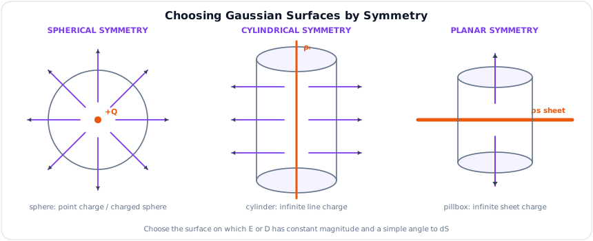
Steps:
- Identify symmetry.
- Choose a Gaussian surface where \(\vec D\) is either constant or perpendicular/parallel to the surface.
- Evaluate \(\oint_S \vec D \cdot d\vec S\).
- Set the result equal to enclosed charge.
- Solve for \(\vec E\) or \(\vec D\).
5. Maxwell's First Equation and Divergence Theorem
Likely Exam Question (10 marks)
"Derive Maxwell's first equation from Gauss' law using the divergence theorem."
Divergence Theorem
The divergence theorem converts a closed surface integral into a volume integral:
Applying this to Gauss' law:
But enclosed charge is:
Using the divergence theorem:
Since this is true for any volume:
This is Maxwell's first equation in point form or Gauss' law in differential form.
For a homogeneous medium:
So:
Meaning of Divergence
Divergence measures the net outward flux per unit volume.
- If \(\nabla \cdot \vec D > 0\), the point acts as a source of flux.
- If \(\nabla \cdot \vec D < 0\), the point acts as a sink of flux.
- If \(\nabla \cdot \vec D = 0\), there is no net source or sink at that point.
6. Standard Results from Gauss' Law
6.1 Infinite Line Charge
For an infinite line charge with density \(\rho_l\) along the \(z\)-axis, choose a cylindrical Gaussian surface of radius \(\rho\) and length \(L\).
By symmetry, \(\vec D = D_\rho\hat a_\rho\) and is constant on the curved surface.
Enclosed charge:
Therefore:
6.2 Infinite Sheet Charge
For an infinite sheet charge with surface density \(\rho_s\), choose a pillbox Gaussian surface crossing the sheet.
Flux leaves through two flat faces:
Enclosed charge:
Therefore:
The field is constant and independent of distance from the sheet.
6.3 Conducting Spherical Shell
For a conducting sphere of radius \(a\) carrying charge \(Q\):
- Inside conductor: \(\vec E = 0\) for \(r < a\).
- Outside conductor: field is same as if all charge were concentrated at the center.
6.4 Uniformly Charged Solid Sphere
Let a solid sphere of radius \(a\) have uniform volume charge density \(\rho_v\).
Total charge:
For \(r < a\), enclosed charge is:
Using Gauss' law:
For \(r \ge a\):
7. Electric Potential
Likely Exam Question (5 or 10 marks)
"Define electric potential and derive the relation between electric field intensity and potential."
Definition
Electric potential at a point is the work done per unit positive charge in bringing the charge from infinity to that point against the electric field.
Unit: volt (V)
Potential Difference
Potential difference between points \(A\) and \(B\) is:
Equivalently:
Relation Between \(\vec E\) and \(V\)
Since electric field points in the direction of maximum decrease of potential:
In Cartesian coordinates:
For one-dimensional variation:
Potential Due to a Point Charge
Taking \(V = 0\) at infinity:
For multiple point charges:
Potential is a scalar quantity, so scalar addition is used instead of vector addition.
Equipotential Surfaces
An equipotential surface is a surface on which potential is constant.
- No work is done moving charge along an equipotential surface.
- Electric field is always normal to an equipotential surface.
- Conductors in electrostatic equilibrium are equipotential bodies.
8. Electrostatic Energy and Capacitance
Likely Exam Question (5 marks)
"Derive the expression for energy stored in an electrostatic field."
Work Done in Assembling Charges
The energy stored in a system of charges is the work required to assemble the charges.
For discrete charges:
For continuous charge distribution:
Energy Density in Electric Field
Energy stored per unit volume in an electric field is:
For a linear medium:
Total energy:
Capacitance
Capacitance is the ability of a conductor system to store charge per unit potential difference.
Unit: farad (F)
For a parallel-plate capacitor:
Energy stored in a capacitor:
9. Laplace and Poisson Equations
Likely Exam Question (10 marks)
"Derive Poisson's and Laplace's equations from Gauss' law. State their physical significance."
Starting with Maxwell's first equation:
For a homogeneous medium:
and:
Therefore:
For constant \(\epsilon\):
Substitute \(\vec E = -\nabla V\):
Hence:
This is Poisson's equation.
If the region is charge-free, \(\rho_v = 0\):
This is Laplace's equation.
Physical Significance
| Equation | Condition | Meaning |
|---|---|---|
| Poisson's equation | Charge exists in region | Potential is produced by volume charge density |
| Laplace's equation | Charge-free region | Potential is determined only by boundary conditions |
Common Forms
Cartesian coordinates:
For one-dimensional variation in \(x\):
In a charge-free one-dimensional region:
So:
and the electric field is uniform:
Boundary Conditions for Electrostatic Fields
At an interface between two media:
| Field Component | Boundary Condition |
|---|---|
| Tangential electric field | \(E_{1t} = E_{2t}\) |
| Normal electric flux density | \(D_{2n} - D_{1n} = \rho_s\) |
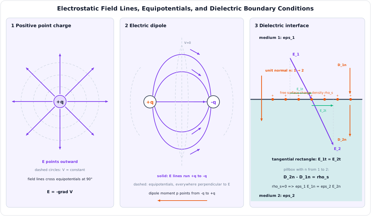
If there is no free surface charge, \(\rho_s = 0\), so:
10. Solved Examples
Example 1 - Field Due to Infinite Line Charge
Q. An infinite line charge has \(\rho_l = 20\,\text{nC/m}\) in free space. Find \(E\) at \(\rho = 5\,\text{cm}\).
Solution:
Direction is radially outward if the line charge is positive.
Example 2 - Potential Difference Between Coaxial Cylinders
Q. Two coaxial conducting cylinders have radii \(a\) and \(b\), where \(b > a\). The inner conductor carries charge density \(\rho_l\). Find the potential difference between them.
Solution:
For \(a < \rho < b\):
Potential difference:
Capacitance per unit length:
Example 3 - Potential from a Given Field
Q. If \(\vec E = 20x\hat a_x\,\text{V/m}\), find the potential difference \(V_A - V_B\) between \(A(1,0,0)\) and \(B(3,0,0)\).
Solution:
Example 4 - Laplace Equation Between Parallel Plates
Q. Two infinite parallel plates at \(x=0\) and \(x=d\) are maintained at \(0\) V and \(V_0\) respectively. Find \(V(x)\) and \(E_x\) in the region between them.
Solution:
The region is charge-free, so:
Hence:
Boundary conditions:
Therefore:
The electric field is uniform and directed from the higher potential plate to the lower potential plate.
11. Quick Revision Table
| Topic | Key Result |
|---|---|
| Coulomb's law | \(F = \frac{1}{4\pi\epsilon}\frac{Q_1Q_2}{R^2}\) |
| Electric field | \(\vec E = \frac{\vec F}{Q_t}\) |
| Point charge field | \(\vec E = \frac{Q}{4\pi\epsilon R^2}\hat a_R\) |
| Electric flux density | \(\vec D = \epsilon\vec E\) |
| Gauss' law | \(\oint_S \vec D \cdot d\vec S = Q_{\text{enc}}\) |
| Maxwell first equation | \(\nabla \cdot \vec D = \rho_v\) |
| Divergence theorem | \(\oint_S \vec A \cdot d\vec S = \int_V \nabla \cdot \vec A\,dv\) |
| Potential-field relation | \(\vec E = -\nabla V\) |
| Energy density | \(w_e = \frac{1}{2}\epsilon E^2\) |
| Poisson equation | \(\nabla^2V = -\rho_v/\epsilon\) |
| Laplace equation | \(\nabla^2V = 0\) |
Key Exam Points - Electrostatics
- Use Coulomb's law for point charges and direct integration for irregular continuous distributions.
- Use Gauss' law only when symmetry makes \(\vec E\) or \(\vec D\) constant over a Gaussian surface.
- Maxwell's first equation is the point form of Gauss' law: \(\nabla \cdot \vec D = \rho_v\).
- Electric field is the negative gradient of potential: \(\vec E = -\nabla V\).
- Poisson equation applies in charge regions; Laplace equation applies in charge-free regions.
Model Answer — Coulomb's Law and Electric Field Intensity [5 marks]
Exam-ready answer
Assume stationary point charges in a homogeneous, linear and isotropic medium of permittivity \(\epsilon\) in farads per metre (F/m). Let \(\vec R_{12}=\vec r_2-\vec r_1\), \(R_{12}=|\vec R_{12}|\), and let \(\hat a_{12}\) point from source charge \(Q_1\) toward \(Q_2\). Coulomb's law states that the force on \(Q_2\) due to \(Q_1\) is
Like charges therefore repel along \(+\hat a_{12}\) and unlike charges attract along \(-\hat a_{12}\). The inverse-square result applies when charge dimensions are negligible compared with separation; for a distributed charge, each differential contribution must be integrated.
Electric field intensity at a point is the force per unit positive test charge as that test charge tends to zero, so it does not disturb the source distribution:
Putting a positive test charge \(q_t\) at distance \(R\) from a source \(Q\) gives
where \(\hat a_R\) is radially outward from \(Q\); the algebraic sign of \(Q\) reverses the direction. By linear superposition,
or the sum becomes \(\int dQ\,\hat a_R/(4\pi\epsilon R^2)\) for line, surface or volume charge.
Check: in free space, \(Q=1\,\mu\text{C}\) at \(R=0.10\,\text{m}\) produces \(E\simeq(8.99\times10^9)(10^{-6})/(0.10)^2=8.99\times10^5\,\text{V/m}\) radially outward. Coulomb's direct formula is unsuitable near material boundaries or for time-varying fields; there one solves the field equations with boundary conditions. Applications include force calculation, electrostatic sensors and the starting field model for capacitance.
Practice target: 8 minutes; define the source-to-field orientation before writing the vector law and finish with units and superposition.
Model Answer — Electric Flux, Flux Density, and the D-E Relation [5 marks]
Exam-ready answer
Electric flux \(\Psi\) measures the total electric displacement crossing an oriented surface. If \(d\vec S=\hat n\,dS\) points outward from a closed surface, then
The sign is positive for flux leaving in the \(+\hat n\) direction and negative for entering flux. Electric flux density or electric displacement \(\vec D\) is flux per unit area normal to the flux; \([\vec D]=\text{C/m}^2\). For a point free charge \(Q\) in a uniform medium, spherical symmetry gives \(\vec D=Q\hat a_r/(4\pi r^2)\).
In matter, the constitutive relation separates free-charge field from material polarization:
where \(\vec P\) is polarization density in C/m\(^2\). For a linear, isotropic dielectric, \(\vec P=\epsilon_0\chi_e\vec E\), hence
Thus \(\vec D\) and \(\vec E\) are parallel only in an isotropic medium. In free space \(\epsilon_r=1\); in an anisotropic dielectric, \(\epsilon\) is a tensor and the vectors need not be parallel.
At an interface whose unit normal \(\hat n\) points from medium 1 to medium 2, an infinitesimal pillbox and loop give
where \(\rho_s\) is free surface charge density in C/m\(^2\). With \(\rho_s=0\), normal \(D\) is continuous while normal \(E\) changes inversely with permittivity.
Check: if \(E=2\,\text{kV/m}\) in a dielectric with \(\epsilon_r=4\), then \(D=\epsilon_0\epsilon_rE=70.8\,\text{nC/m}^2\). In a uniform capacitor, \(C=Q/V\), \(D=Q/A\), and stored energy density is \(w_e=\tfrac12\vec E\cdot\vec D\) J/m\(^3\). These relations support capacitor and insulation design, but nonlinear or hysteretic dielectrics require their measured \(D\)-\(E\) law.
Practice target: 8–9 minutes; show the outward surface normal, both constitutive forms, units, and the two interface conditions.
Model Answer — Gauss's Law and Maxwell's First Equation [10 marks]
Exam-ready answer
Let \(S\) be a closed surface bounding volume \(V\), with \(d\vec S=\hat n\,dS\) directed outward. Gauss's law states that the net outward electric displacement flux equals the enclosed free charge:
where \(\vec D\) is in C/m\(^2\), \(\rho_v\) is free volume-charge density in C/m\(^3\), and \(Q_{\text{enc}}\) is in coulombs. Charges outside \(S\) can produce local flux, but their entering and leaving contributions cancel in the net integral.
The divergence theorem converts the flux of any differentiable vector field through a closed surface into a volume integral:
Combining this with Gauss's law gives
Because the equality holds for every arbitrary infinitesimal volume, the integrands must be equal:
This is Maxwell's first equation in differential or point form. It says that positive free charge is a source of \(\vec D\), negative free charge is a sink, and a charge-free point has zero net local divergence. For a homogeneous linear dielectric, \(\vec D=\epsilon\vec E\), so \(\nabla\cdot\vec E=\rho_v/\epsilon\); if \(\epsilon\) varies spatially, one must retain \(\nabla\cdot(\epsilon\vec E)=\rho_v\) rather than pulling \(\epsilon\) outside the divergence.
Symmetry check: enclose a positive point charge \(Q\) by a sphere of radius \(r\). The field is radial and has constant magnitude on the sphere, so
The outward direction follows from \(Q>0\); a negative \(Q\) reverses it. The \(1/r^2\) decrease exactly offsets the \(4\pi r^2\) growth of spherical area, leaving total flux equal to \(Q\).
Across a dielectric boundary, the same law applied to a vanishing pillbox whose normal points from region 1 to 2 gives \(\hat n\cdot(\vec D_2-\vec D_1)=\rho_s\). This is the surface-charge counterpart of the volume equation and is essential in capacitor and dielectric-interface problems.
Gauss's law is universally valid in electrostatics, but it is an efficient field-solving tool only for spherical, cylindrical or planar symmetry, where the normal component is constant or zero on chosen surface pieces. For arbitrary geometry it still checks flux and charge conservation, while Poisson/Laplace methods or numerical field solvers determine \(\vec E\). Applications include coaxial capacitance, charged conductors, dielectric boundaries and verification of finite-element solutions.
Practice target: 16–18 minutes; reserve one-third for the integral-to-differential derivation and draw the symmetry-matched Gaussian surfaces.
Model Answer — Fields from Point, Line, and Spherical Charges [5 marks]
Exam-ready answer
Assume an infinite homogeneous medium of permittivity \(\epsilon\) and use outward-oriented Gaussian surfaces. Gauss's law is
1. Point charge \(Q\). Choose a concentric sphere of radius \(r\). Spherical symmetry makes \(\vec D=D_r\hat a_r\) constant and normal to the surface:
2. Infinite line charge \(\lambda\) C/m. Choose a coaxial cylinder of radius \(\rho\) and length \(L\). Flux through the end caps is zero because \(\vec D=D_\rho\hat a_\rho\) is parallel to them. Therefore
3. Uniformly charged solid sphere. Let its radius be \(a\) and volume density be \(\rho_v\) C/m\(^3\). For \(r<a\), the enclosed charge is \(\rho_v(4\pi r^3/3)\); for \(r\ge a\), the total charge is \(Q=\rho_v4\pi a^3/3\). Hence
For a conducting sphere or thin spherical shell in electrostatic equilibrium, \(E=0\) inside and the outside expression is unchanged. Positive \(Q\), \(\lambda\) or \(\rho_v\) gives outward fields; negative charge reverses each unit vector.
Check: the solid-sphere formulas agree at \(r=a\), both giving \(E(a)=\rho_v a/(3\epsilon)\), so there is no discontinuity when no surface-charge sheet is present. The three decays differ because enclosed charge and Gaussian area scale differently: \(1/r^2\) for a localized charge, \(1/\rho\) for a line, and linear growth inside a uniform sphere. These ideal results model conductors and coaxial systems; finite lines or nonspherical charge distributions lack the assumed symmetry and require Coulomb integration or numerical solution.
Practice target: 9 minutes; draw all three Gaussian surfaces and show the enclosed-charge step for the solid sphere.
Model Answer — Electric Potential and the Field-Gradient Relation [5 marks]
Exam-ready answer
In electrostatics, \(\nabla\times\vec E=0\), so the field is conservative and work is path independent. The potential difference from point \(A\) to point \(B\) is the negative work done by the electric field per unit positive test charge:
The minus sign means potential decreases when \(d\vec l\) points along \(\vec E\). Equivalently, the external work per unit charge in a quasistatic displacement is \(+\Delta V\). For two neighboring points separated by \(d\vec l\),
But the total differential of a scalar field is \(dV=\nabla V\cdot d\vec l\). Since this equality holds for every displacement direction,
Thus \(\vec E\) is normal to an equipotential surface and points toward the greatest decrease of \(V\); no work is done along an equipotential. With reference \(V(\infty)=0\), integration of the radial point-charge field gives
Check: differentiating this result yields \(E_r=-dV/dr=Q/(4\pi\epsilon r^2)\), outward for \(Q>0\), confirming both sign and units. Potential is a scalar and therefore usually easier to superpose than vector fields: \(V=\sum_iQ_i/(4\pi\epsilon R_i)\), followed by \(\vec E=-\nabla V\).
The relation is used in boundary-value, capacitor and insulation calculations. If two conductors carry \(\pm Q\) at potential difference \(V\), \(C=Q/V\) in farads and stored energy is \(W=\tfrac12CV^2=\tfrac12QV\) joules. Absolute potential depends on the chosen reference, whereas potential difference and \(\vec E\) are physical. The electrostatic scalar-potential description alone is insufficient for a general time-varying magnetic vector potential, where \(\vec E=-\nabla V-\partial\vec A/\partial t\).
Practice target: 8 minutes; state whose work fixes the sign, derive the gradient relation, and verify it with the point-charge potential.
Model Answer — Poisson's and Laplace's Equations [5 marks]
Exam-ready answer
For an electrostatic field, Maxwell's first equation and the potential relation are
where \(\rho_v\) is free charge density in C/m\(^3\), \(V\) is potential in volts and \(\vec E\) is in V/m. In a linear medium \(\vec D=\epsilon\vec E\). Substitution, with the gradient orientation chosen so \(\vec E\) points from high to low potential, gives the general material equation
If \(\epsilon\) is constant, it can be taken outside the divergence:
In a charge-free region, \(\rho_v=0\), so
In Cartesian coordinates, \(\nabla^2V=\partial^2V/\partial x^2+\partial^2V/\partial y^2+\partial^2V/\partial z^2\). Poisson's equation describes regions containing charge; Laplace's equation determines source-free fields from boundary values. A unique solution follows when conductor potentials are specified (Dirichlet data), normal field or charge is specified (Neumann data), or compatible mixed data are supplied. At a dielectric interface, \(V\) and tangential \(E\) are continuous, while \(\hat n\cdot(\vec D_2-\vec D_1)=\rho_s\) for a normal directed from medium 1 to 2.
Worked check: parallel plates. Let \(V(0)=0\) and \(V(d)=V_0\) in a charge-free uniform dielectric. One-dimensional Laplace equation gives \(d^2V/dx^2=0\), hence \(V=Ax+B\). Applying the boundaries yields
For plate area \(A\) with negligible fringing, \(C=\epsilon A/d\) F, \(W=\tfrac12CV_0^2\) J and \(w_e=\tfrac12\epsilon E^2\) J/m\(^3\). Applications include capacitors, coaxial cables, shielding and semiconductor depletion regions. The simple constant-\(\epsilon\) Poisson form is not valid across abrupt or nonlinear material changes; use \(\nabla\cdot(\epsilon\nabla V)=-\rho_v\) piecewise with the interface conditions, often numerically for irregular geometry.
Practice target: 9 minutes; derive both equations before using the plate boundary conditions to check the sign of the field.